Biplot

Biplot

Usage

# S4 method for CA
biplot(
  x,
  ...,
  axes = c(1, 2),
  type = c("symetric", "rows", "columns", "contributions"),
  active = TRUE,
  sup = TRUE,
  labels = NULL,
  col.rows = c("#E69F00", "#009E73"),
  col.columns = c("#56B4E9", "#F0E442"),
  cex.rows = graphics::par("cex"),
  cex.columns = graphics::par("cex"),
  pch.rows = 16,
  pch.columns = 17,
  xlim = NULL,
  ylim = NULL,
  main = NULL,
  sub = NULL,
  legend = list(x = "topleft")
)

# S4 method for PCA
biplot(
  x,
  ...,
  axes = c(1, 2),
  type = c("form", "covariance"),
  active = TRUE,
  sup = TRUE,
  labels = "variables",
  col.rows = c("#E69F00", "#009E73"),
  col.columns = c("#56B4E9", "#F0E442"),
  pch = 16,
  cex = 1,
  lty = 1,
  lwd = 2,
  xlim = NULL,
  ylim = NULL,
  main = NULL,
  sub = NULL,
  legend = list(x = "topleft")
)

Arguments

x: A CA, MCA or PCA object.
...: Currently not used.
axes: A length-two numeric vector giving the dimensions to be plotted.
type: A character string specifying the biplot to be plotted (see below). It must be one of "rows", "columns", "contribution" (CA), "form" or "covariance" (PCA). Any unambiguous substring can be given.
active: A logical scalar: should the active observations be plotted?
sup: A logical scalar: should the supplementary observations be plotted?
labels: A character vector specifying whether "rows"/"individuals" and/or "columns"/"variables" names must be drawn. Any unambiguous substring can be given.
col.rows: A length-two vector of color specification for the active and supplementary rows.
col.columns: A length-two vector of color specification for the active and supplementary columns.
xlim: A length-two numeric vector giving the x limits of the plot. The default value, NULL, indicates that the range of the finite values to be plotted should be used.
ylim: A length-two numeric vector giving the y limits of the plot. The default value, NULL, indicates that the range of the finite values to be plotted should be used.
main: A character string giving a main title for the plot.
sub: A character string giving a subtitle for the plot.
legend: A list of additional arguments to be passed to graphics::legend(); names of the list are used as argument names. If NULL, no legend is displayed.
pch, pch.rows, pch.columns: A symbol specification.
cex, cex.rows, cex.columns: A numeric vector giving the amount by which plotting characters and symbols should be scaled relative to the default.
lty, lwd: A specification for the line type and width.

Value

biplot() is called for its side-effects: it results in a graphic being displayed. Invisibly returns x.

Details

A biplot is the simultaneous representation of rows and columns of a rectangular dataset. It is the generalization of a scatterplot to the case of mutlivariate data: it allows to visualize as much information as possible in a single graph (Greenacre 2010).

Biplots have the drawbacks of their advantages: they can quickly become difficult to read as they display a lot of information at once. It may then be preferable to visualize the results for individuals and variables separately.

PCA Biplots

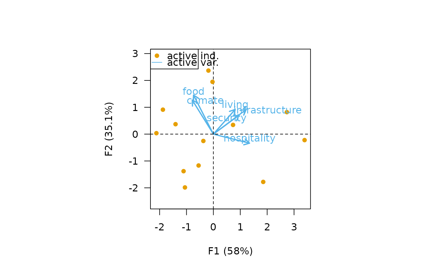
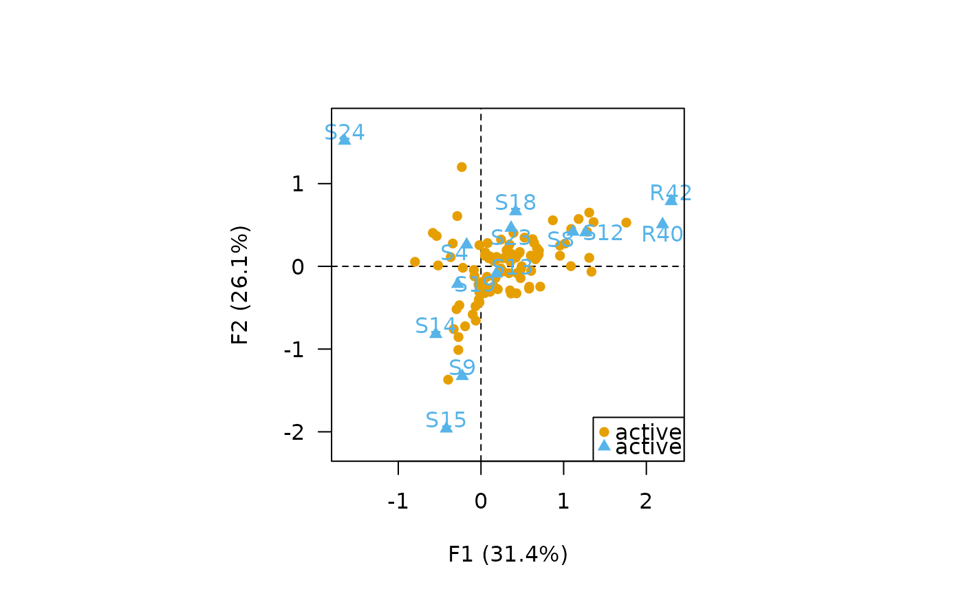
form (row-metric-preserving): The form biplot favors the representation of the individuals: the distance between the individuals approximates the Euclidean distance between rows. In the form biplot the length of a vector approximates the quality of the representation of the variable.
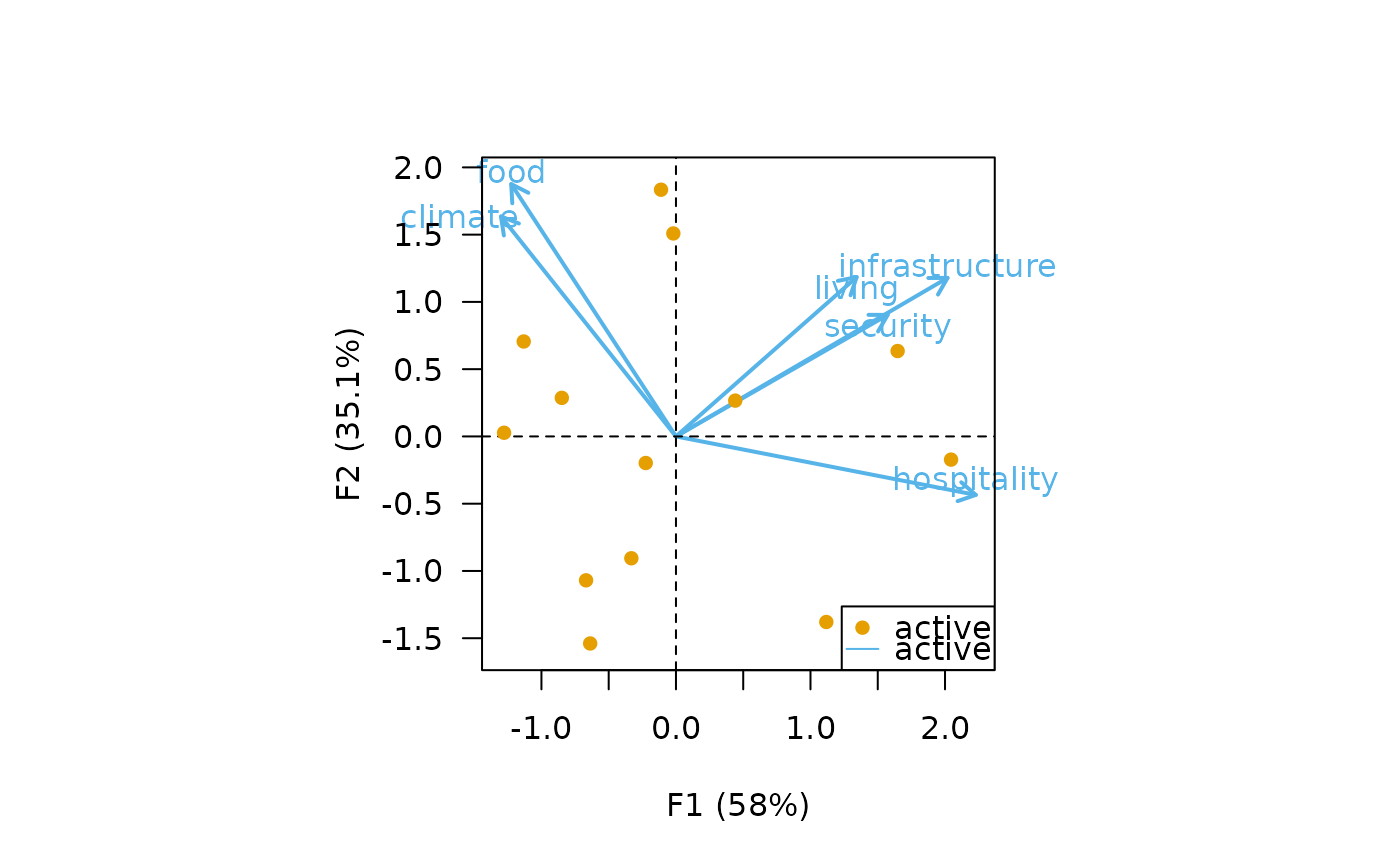
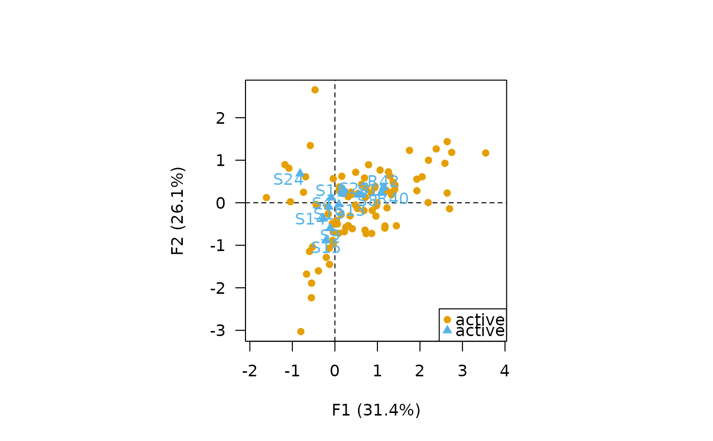
covariance (column-metric-preserving): The covariance biplot favors the representation of the variables: the length of a vector approximates the standard deviation of the variable and the cosine of the angle formed by two vectors approximates the correlation between the two variables. In the covariance biplot the distance between the individuals approximates the Mahalanobis distance between rows.

CA Biplots

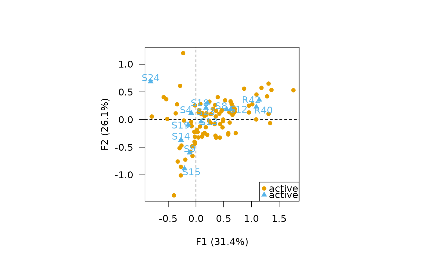
symetric (symetric biplot): Represents the row and column profiles simultaneously in a common space: rows and columns are in standard coordinates. Note that the the inter-distance between any row and column items is not meaningful.
rows (asymetric biplot): Row principal biplot (row-metric-preserving) with rows in principal coordinates and columns in standard coordinates.
columns (asymetric biplot): Column principal biplot (column-metric-preserving) with rows in standard coordinates and columns in principal coordinates.
contribution (asymetric biplot): Contribution biplot with rows in principal coordinates and columns in standard coordinates multiplied by the square roots of their masses.

References

Aitchison, J. and Greenacre, M. J. (2002). Biplots of Compositional Data. Journal of the Royal Statistical Society: Series C (Applied Statistics), 51(4): 375-92. doi:10.1111/1467-9876.00275 .

Greenacre, M. J. (2010). Biplots in Practice. Bilbao: Fundación BBVA.

Author

N. Frerebeau

Examples

## Replicate examples from Greenacre 2007, p. 59-68
data("countries")

## Compute principal components analysis
## All rows and all columns obtain the same weight
row_w <- rep(1 / nrow(countries), nrow(countries)) # 1/13
col_w <- rep(1 / ncol(countries), ncol(countries)) # 1/6
Y <- pca(countries, scale = FALSE, weight_row = row_w, weight_col = col_w)

## Row-metric-preserving biplot (form biplot)
biplot(Y, type = "form")


## Column-metric-preserving biplot (covariance biplot)
biplot(Y, type = "covariance", legend = list(x = "bottomright"))


## Replicate examples from Greenacre 2007, p. 79-88
data("benthos")

## Compute correspondence analysis
X <- ca(benthos)

## Symetric CA biplot
biplot(X, labels = "columns", legend = list(x = "bottomright"))


## Row principal CA biplot
biplot(X, type = "row", labels = "columns", legend = list(x = "bottomright"))


## Column principal CA biplot
biplot(X, type = "column", labels = "columns", legend = list(x = "bottomright"))


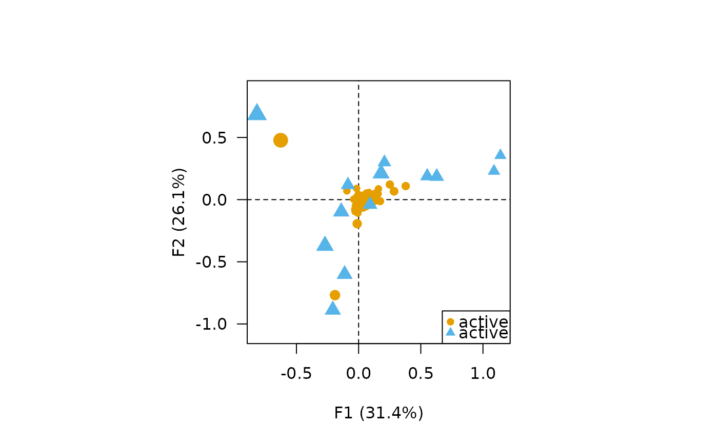
## Contribution CA biplot
biplot(X, type = "contrib", labels = NULL, legend = list(x = "bottomright"))