## Load data
data("XRD") # X-ray diffraction

## Subset from 20 to 70 degrees
XRD <- signal_select(XRD, from = 20, to = 70)

## Y plot limits
ylim <- c(0, max(XRD$y))
Linear baseline
## Plot spectrum
plot(XRD, type = "l", ylim = ylim, xlab = expression(2*theta), ylab = "Count")
abline(h = 0, lty = "dashed")

## Estimate the baseline between 25 and 34 degrees
baseline <- baseline_linear(XRD, points = c(25, 34))

## Plot the baseline
lines(baseline, col = "red")

## Correct spectrum
corrected <- signal_drift(XRD, lag = baseline, subtract = TRUE)

lines(corrected, col = "blue")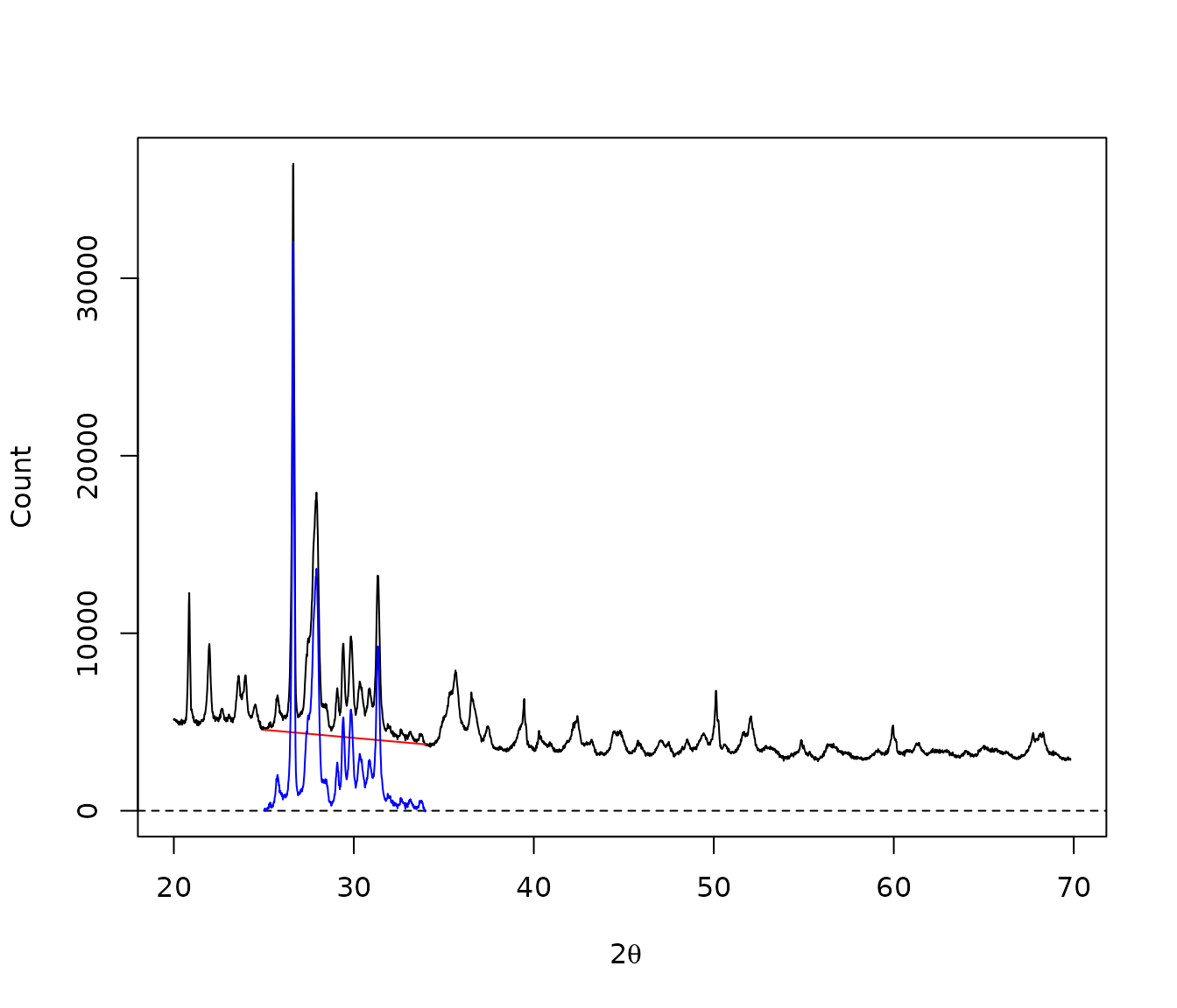
Linear baseline.
Polynomial baseline
## Plot spectrum
plot(XRD, type = "l", ylim = ylim, xlab = expression(2*theta), ylab = "Count")
abline(h = 0, lty = "dashed")

## Estimate the baseline
baseline <- baseline_polynomial(XRD, d = 4, tolerance = 0.02, stop = 1000)

## Plot the baseline
lines(baseline, col = "red")

## Correct spectrum
corrected <- signal_drift(XRD, lag = baseline, subtract = TRUE)

lines(corrected, col = "blue")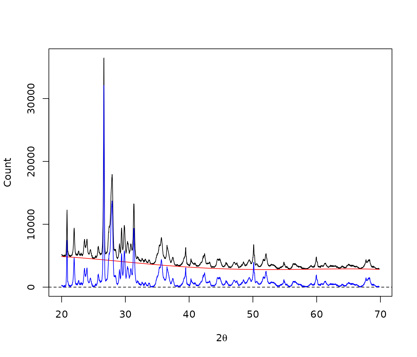
Polynomial baseline.
Asymmetric Least Squares Smoothing
## Plot spectrum
plot(XRD, type = "l", ylim = ylim, xlab = "Energy (keV)", ylab = "Count")
abline(h = 0, lty = "dashed")

## AsLS baseline
baseline <- baseline_asls(XRD, p = 0.005, lambda = 10^7)

## Plot the baseline
lines(baseline, col = "red")

## Correct spectrum
corrected <- signal_drift(XRD, lag = baseline, subtract = TRUE)

lines(corrected, col = "blue")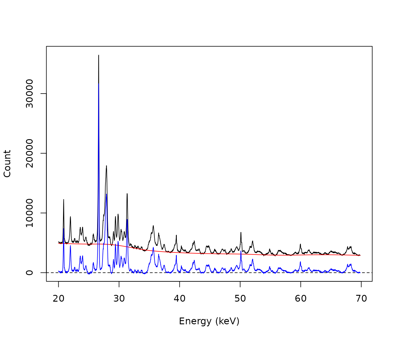
Asymmetric Least Squares Smoothing.
Rolling Ball baseline
## Plot spectrum
plot(XRD, type = "l", ylim = ylim, xlab = expression(2*theta), ylab = "Count")
abline(h = 0, lty = "dashed")

## Estimate the baseline
baseline <- baseline_rollingball(XRD, m = 201, s = 151)

## Plot the baseline
lines(baseline, col = "red")

## Correct spectrum
corrected <- signal_drift(XRD, lag = baseline, subtract = TRUE)

lines(corrected, col = "blue")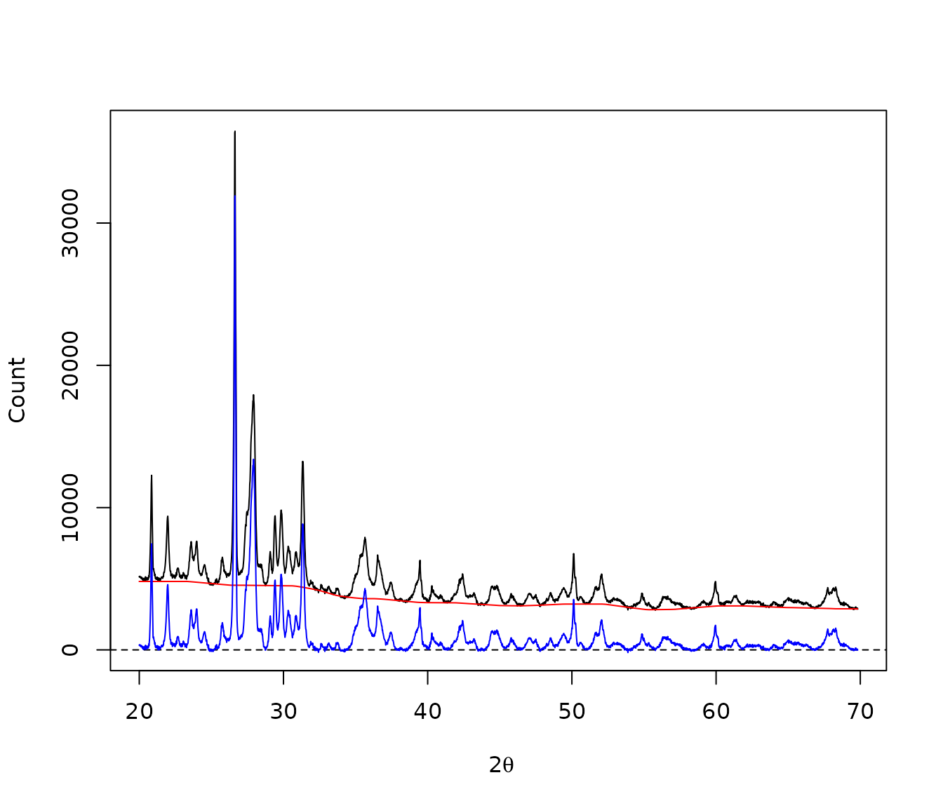
Rolling Ball baseline.
Rubberband baseline
## Plot spectrum
plot(XRD, type = "l", ylim = ylim, xlab = expression(2*theta), ylab = "Count")
abline(h = 0, lty = "dashed")

## Estimate the baseline
baseline <- baseline_rubberband(XRD)

## Plot the baseline
lines(baseline, col = "red")

## Correct spectrum
corrected <- signal_drift(XRD, lag = baseline, subtract = TRUE)

lines(corrected, col = "blue")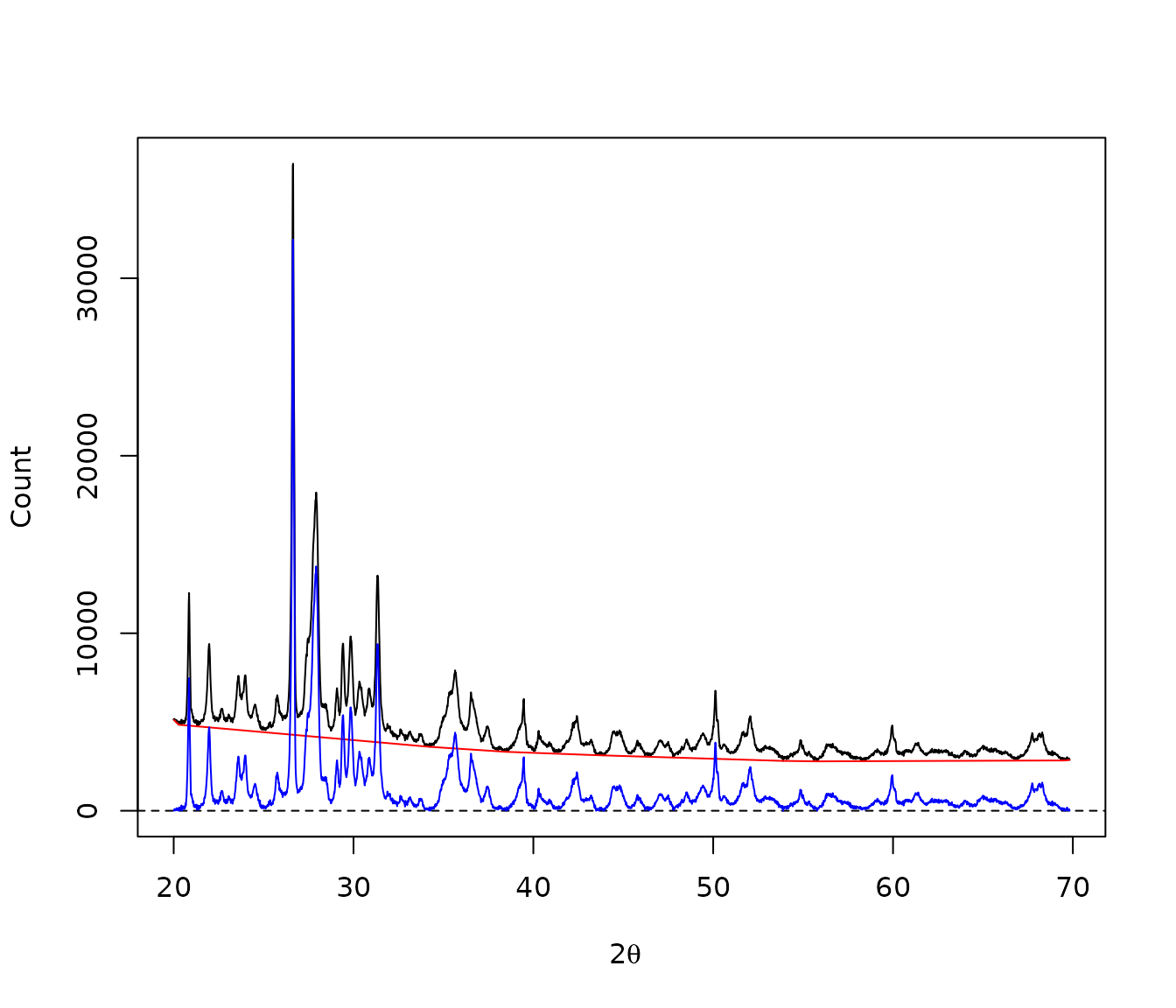
Rubberband baseline.
SNIP baseline
## Plot spectrum
plot(XRD, type = "l", ylim = ylim, xlab = expression(2*theta), ylab = "Count")
abline(h = 0, lty = "dashed")

## Estimate the baseline
baseline <- baseline_snip(XRD, LLS = FALSE, decreasing = FALSE, n = 100)

## Plot the baseline
lines(baseline, col = "red")

## Correct spectrum
corrected <- signal_drift(XRD, lag = baseline, subtract = TRUE)

lines(corrected, col = "blue")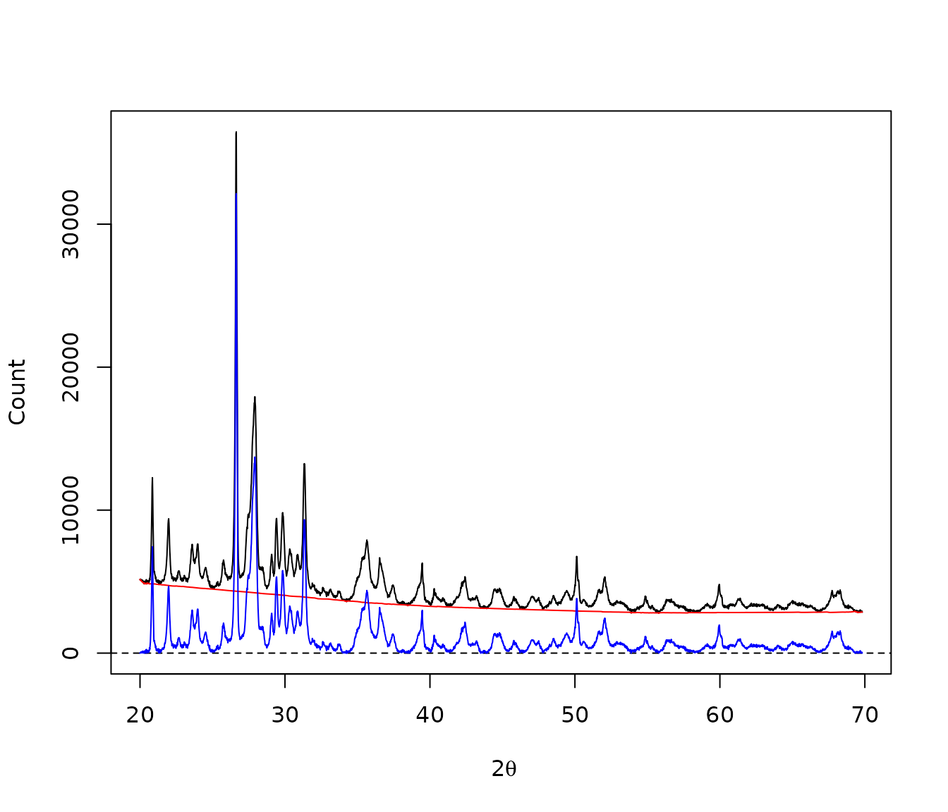
SNIP baseline.
4S Peak Filling
## Plot spectrum
plot(XRD, type = "l", ylim = ylim, xlab = "Energy (keV)", ylab = "Count")
abline(h = 0, lty = "dashed")

## 4S Peak Filling baseline
baseline <- baseline_peakfilling(XRD, n = 10, m = 5, by = 10,
                                 lambda = 1000, d = 3, sparse = TRUE)

## Plot the baseline
lines(baseline, col = "red")

## Correct spectrum
corrected <- signal_drift(XRD, lag = baseline, subtract = TRUE)

lines(corrected, col = "blue")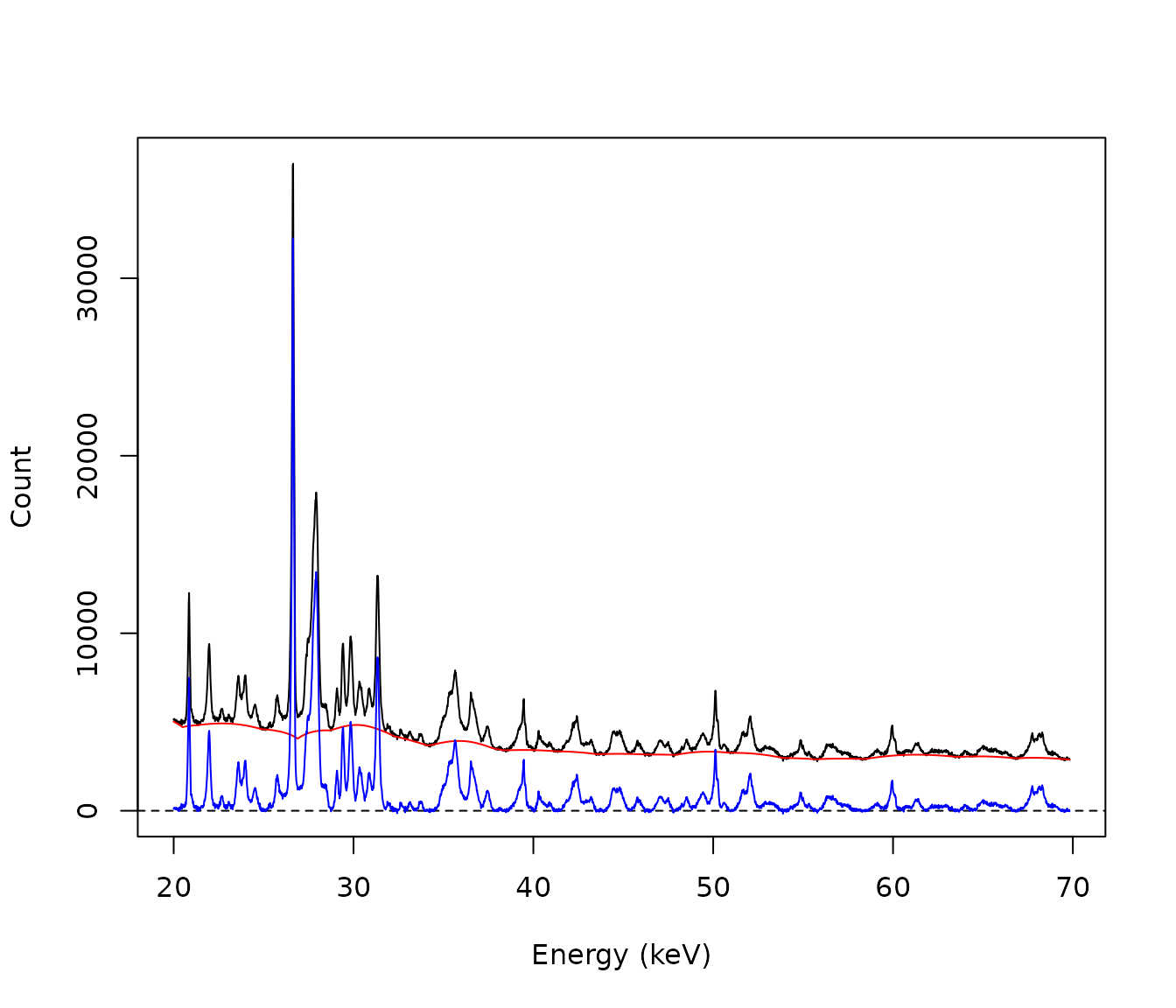
4S Peak Filling.