Event Date Model

## Install extra packages (if needed):
# install.packages("folio") # datasets

# Load packages
library(kairos)
#> Loading required package: dimensio

Definition

Event and accumulation dates are density estimates of the occupation and duration of an archaeological site (Bellanger, Husi and Tomassone 2006; Bellanger, Tomassone and Husi 2008; Bellanger and Husi 2012).

The event date is an estimation of the terminus post-quem of an archaeological assemblage. The accumulation date represents the “chronological profile” of the assemblage. According to Bellanger and Husi (2012), accumulation date can be interpreted “at best […] as a formation process reflecting the duration or succession of events on the scale of archaeological time, and at worst, as imprecise dating due to contamination of the context by residual or intrusive material.” In other words, accumulation dates estimate occurrence of archaeological events and rhythms of the long term.

Event Date

Event dates are estimated by fitting a Gaussian multiple linear regression model on the factors resulting from a correspondence analysis - somewhat similar to the idea introduced by Poblome and Groenen (2003). This model results from the known dates of a selection of reliable contexts and allows to predict the event dates of the remaining assemblages.

First, a correspondence analysis (CA) is carried out to summarize the information in the count matrix $X$ . The correspondence analysis of $X$ provides the coordinates of the $m$ rows along the $q$ factorial components, denoted $f_{ik} ~\forall i \in \left[ 1,m \right], k \in \left[ 1,q \right]$ .

Then, assuming that $n$ assemblages are reliably dated by another source, a Gaussian multiple linear regression model is fitted on the factorial components for the $n$ dated assemblages:

$t^E_i = \beta_{0} + \sum_{k = 1}^{q} \beta_{k} f_{ik} + \epsilon_i ~\forall i \in [1,n]$ where $t^E_i$ is the known date point estimate of the $i$ th assemblage, $\beta_k$ are the regression coefficients and $\epsilon_i$ are normally, identically and independently distributed random variables, $\epsilon_i \sim \mathcal{N}(0,\sigma^2)$ .

These $n$ equations are stacked together and written in matrix notation as

$t^E = F \beta + \epsilon$

where $\epsilon \sim \mathcal{N}_{n}(0,\sigma^2 I_{n})$ , $\beta = \left[ \beta_0 \cdots \beta_q \right]' \in \mathbb{R}^{q+1}$ and

$F = \begin{bmatrix} 1 & f_{11} & \cdots & f_{1q} \\ 1 & f_{21} & \cdots & f_{2q} \\ \vdots & \vdots & \ddots & \vdots \\ 1 & f_{n1} & \cdots & f_{nq} \end{bmatrix}$

Assuming that $F'F$ is nonsingular, the ordinary least squares estimator of the unknown parameter vector $\beta$ is:

$\widehat{\beta} = \left( F'F \right)^{-1} F' t^E$

Finally, for a given vector of CA coordinates $f_i$ , the predicted event date of an assemblage $t^E_i$ is:

$\widehat{t^E_i} = f_i \hat{\beta}$

The endpoints of the $100(1 − \alpha)$ % associated prediction confidence interval are given as:

$\widehat{t^E_i} \pm t_{\alpha/2,n-q-1} \sqrt{\widehat{V}}$

where $\widehat{V_i}$ is an estimator of the variance of the prediction error: $\widehat{V_i} = \widehat{\sigma}^2 \left( f_i^T \left( F'F \right)^{-1} f_i + 1 \right)$

were $\widehat{\sigma} = \frac{\sum_{i=1}^{n} \left( t_i - \widehat{t^E_i} \right)^2}{n - q - 1}$ .

The probability density of an event date $t^E_i$ can be described as a normal distribution:

$t^E_i \sim \mathcal{N}(\widehat{t^E_i},\widehat{V_i})$

Accumulation Date

As row (assemblages) and columns (types) CA coordinates are linked together through the so-called transition formulae, event dates for each type $t^E_j$ can be predicted following the same procedure as above.

Then, the accumulation date $t^A_i$ is defined as the weighted mean of the event date of the ceramic types found in a given assemblage. The weights are the conditional frequencies of the respective types in the assemblage (akin to the MCD).

The accumulation date is estimated as: $\widehat{t^A_i} = \sum_{j = 1}^{p} \widehat{t^E_j} \times \frac{x_{ij}}{x_{i \cdot}}$

The probability density of an accumulation date $t^A_i$ can be described as a Gaussian mixture:

$t^A_i \sim \frac{x_{ij}}{x_{i \cdot}} \mathcal{N}(\widehat{t^E_j},\widehat{V_j}^2)$

Interestingly, the integral of the accumulation date offers an estimates of the cumulative occurrence of archaeological events, which is close enough to the definition of the tempo plot introduced by Dye (2016).

Limitation

Event and accumulation dates estimation relies on the same conditions and assumptions as the matrix seriation problem. Dunnell (1970) summarizes these conditions and assumptions as follows.

The homogeneity conditions state that all the groups included in a seriation must:

Be of comparable duration.
Belong to the same cultural tradition.
Come from the same local area.

The mathematical assumptions state that the distribution of any historical or temporal class:

Is continuous through time.
Exhibits the form of a unimodal curve.

Theses assumptions create a distributional model and ordering is accomplished by arranging the matrix so that the class distributions approximate the required pattern. The resulting order is inferred to be chronological.

Predicted dates have to be interpreted with care: these dates are highly dependent on the range of the known dates and the fit of the regression.

Usage

This package provides an implementation of the chronological modeling method developed by Bellanger and Husi (2012). This method is slightly modified here and allows the construction of different probability density curves of archaeological assemblage dates (event, activity and tempo).

## Bellanger et al. did not publish the data supporting their demonstration: 
## no replication of their results is possible. 
## Here is an example using the Zuni dataset from Peeples and Schachner 2012
data("zuni", package = "folio")

## Assume that some assemblages are reliably dated (this is NOT a real example)
## The names of the vector entries must match the names of the assemblages
zuni_dates <- c(
  LZ0569 = 1097, LZ0279 = 1119, CS16 = 1328, LZ0066 = 1111,
  LZ0852 = 1216, LZ1209 = 1251, CS144 = 1262, LZ0563 = 1206,
  LZ0329 = 1076, LZ0005Q = 859, LZ0322 = 1109, LZ0067 = 863,
  LZ0578 = 1180, LZ0227 = 1104, LZ0610 = 1074
)

## Model the event and accumulation date for each assemblage
model <- event(zuni, dates = zuni_dates, rank = 10)

## Model summary
## (results are expressed in rata die)
summary(model)
#> 
#> Call:
#> stats::lm(formula = date ~ ., data = contexts)
#> 
#> Residuals:
#>   LZ0852   LZ0610   LZ0578   LZ0569   LZ0563   LZ0329   LZ0322   LZ0279 
#>  -479.32   351.48  1283.51   163.57 -1626.71  -290.90   950.04 -1427.33 
#>   LZ0227   LZ0067   LZ0066  LZ0005Q     CS16    CS144   LZ1209 
#>  -280.59   -50.24   266.02    45.83  -105.47  1016.24   183.86 
#> attr(,"class")
#> [1] "RataDie"
#> attr(,"class")attr(,"package")
#> [1] "aion"
#> 
#> Coefficients:
#>             Estimate Std. Error t value Pr(>|t|)    
#> (Intercept) 425015.4     1064.9 399.095 2.36e-10 ***
#> F1          -57813.4      602.6 -95.938 7.08e-08 ***
#> F2            9387.7      615.2  15.260 0.000108 ***
#> F3           -2047.2      789.1  -2.594 0.060411 .  
#> F4            3928.9     2127.1   1.847 0.138452    
#> F5           -1146.2     1442.3  -0.795 0.471276    
#> F6             995.1      485.4   2.050 0.109663    
#> F7            1667.0     1906.7   0.874 0.431304    
#> F8            4126.0     1264.9   3.262 0.031027 *  
#> F9           -1889.1     1079.6  -1.750 0.155039    
#> F10           -144.8      967.9  -0.150 0.888300    
#> ---
#> Signif. codes:  0 '***' 0.001 '**' 0.01 '*' 0.05 '.' 0.1 ' ' 1
#> 
#> Residual standard error: 1494 on 4 degrees of freedom
#> Multiple R-squared:  0.9997, Adjusted R-squared:  0.999 
#> F-statistic:  1433 on 10 and 4 DF,  p-value: 1.168e-06

## Extract model coefficients
## (convert results to Gregorian years)
coef(model, calendar = CE())
#>  (Intercept)           F1           F2           F3           F4           F5 
#> 1163.6512430 -158.2887134   25.7005062   -5.6059619   10.7559523   -3.1402928 
#>           F6           F7           F8           F9          F10 
#>    2.7236281    4.5617156   11.2951729   -5.1728421   -0.3984238

## Extract residual standard deviation
## (convert results to Gregorian years)
sigma(model, calendar = CE())
#> [1] 4.088072

## Extract model residuals
## (convert results to Gregorian years)
resid(model, calendar = CE())
#>  [1] -1.3132066  0.9602214  3.5123344  0.4453877 -4.4554781 -0.7975492
#>  [7]  2.6001038 -3.9104984 -0.7693659 -0.1399926  0.7260925  0.1228117
#> [13] -0.2908912  2.7814906  0.5009809

## Extract model fitted values
## (convert results to Gregorian years)
fitted(model, calendar = CE())
#>  [1] 1217.3105 1073.0370 1176.4849 1096.5531 1210.4540 1076.7948 1106.3999
#>  [8] 1122.9078 1104.7666  863.1376 1110.2712  858.8744 1328.2882 1259.2185
#> [15] 1250.4963

## Estimate event dates
## (results are expressed in rata die)
eve <- predict_event(model, margin = 1, level = 0.95)
head(eve)
#>            date    lower    upper    error
#> LZ1105 426454.0 420445.5 432462.4 2164.087
#> LZ1103 417145.8 414689.9 419601.7  884.558
#> LZ1100 421968.1 416394.9 427541.4 2007.317
#> LZ1099 400974.7 396642.1 405307.4 1560.503
#> LZ1097 397176.5 393404.6 400948.3 1358.530
#> LZ1096 306371.0 300801.2 311940.7 2006.057

## Activity plot
plot(model, type = "activity", event = TRUE, select = 1:6)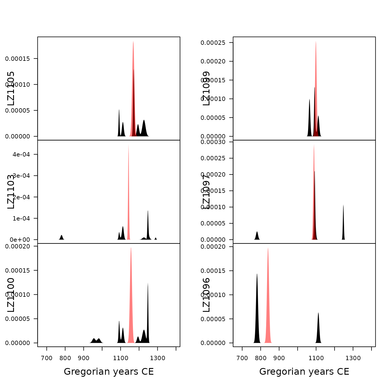

plot(model, type = "activity", event = TRUE, select = "LZ1105")


## Tempo plot
plot(model, type = "tempo", select = "LZ1105")

Resampling methods can be used to check the stability of the resulting model. If jackknife() is used, one type/fabric is removed at a time and all statistics are recalculated. In this way, one can assess whether certain type/fabric has a substantial influence on the date estimate. If bootstrap() is used, a large number of new bootstrap assemblages is created, with the same sample size, by resampling the original assemblage with replacement. Then, examination of the bootstrap statistics makes it possible to pinpoint assemblages that require further investigation.

## Check model variability
## (results are expressed in rata die)
## Warning: this may take a few seconds

## Jackknife fabrics
jack <- jackknife(model)
head(jack)
#>             date     lower     upper    error       bias
#> LZ1105 155634807 155628798 155640815 2164.087 2638541997
#> LZ1103 152396320 152393864 152398776  884.558 2583645955
#> LZ1100 154171872 154166299 154177445 2007.317 2613748366
#> LZ1099 146238877 146234544 146243210 1560.503 2479244339
#> LZ1097 145631868 145628096 145635640 1358.530 2468989755
#> LZ1096 112226452 112220882 112232021 2006.057 1902641373

## Bootstrap of assemblages
boot <- bootstrap(model, n = 30)
head(boot)
#>             min     mean      max       Q5      Q95
#> LZ1105 414363.1 426390.3 451574.2 415670.7 436649.5
#> LZ1103 403049.1 420746.5 435898.2 408015.7 433293.7
#> LZ1100 396645.1 418561.3 430966.4 399416.5 429908.2
#> LZ1099 397468.8 400799.6 405836.6 397962.2 403957.1
#> LZ1097 364251.8 395040.1 429251.0 367933.7 420697.8
#> LZ1096 264824.9 301692.1 354308.8 264824.9 337530.5

References

Bellanger, L., Husi, P. & Tomassone, R. (2006). Une approche statistique pour la datation de contextes archéologiques. Revue de statistique appliquée, 54(2), 65-81. URL: http://www.numdam.org/item/RSA_2006__54_2_65_0/.

Bellanger, L. & Husi, P. (2012). Statistical Tool for Dating and Interpreting Archaeological Contexts Using Pottery. Journal of Archaeological Science, 39(4), 777-790. DOI: 10.1016/j.jas.2011.06.031.

Bellanger, L. & Tomassone, R. & Husi, P. (2008). A Statistical Approach for Dating Archaeological Contexts. Journal of Data Science, 6, 135-154.

Dunnell, R. C. (1970). Seriation Method and Its Evaluation. American Antiquity, 35(3), 305-319. DOI: 10.2307/278341.

Dye, T. S. (2016). Long-Term Rhythms in the Development of Hawaiian Social Stratification. Journal of Archaeological Science, 71, 1-9. DOI: 10.1016/j.jas.2016.05.006.

Poblome, J. & Groenen, P. J. F. (2003). Constrained Correspondence Analysis for Seriation of Sagalassos Tablewares. In M. Doerr & A. Sarris (Eds.), The Digital Heritage of Archaeology Athens: Hellenic Ministry of Culture.