Base R ships with a lot of functionality useful for time series, in particular in the stats package. However, these features are not adapted to most archaeological time series. These are indeed defined for a given calendar era, they can involve dates very far in the past and the sampling of the observation time is (in most cases) not constant. aion provides a system of classes and methods to represent and work with such time-series.
Calendars
aion currently supports both Julian and Gregorian
calendars (with the most common eras for the latter, e.g. Before
Present, Common Era…). A calendar can be defined using the
calendar() function:
## Create a calendar object
## (Gregorian Common Era)
calendar("CE")
#> Common Era (CE): Gregorian years counted forwards from 0
Or by using the shortcuts:
## Common Era (Gregorian)
CE()
#> Common Era (CE): Gregorian years counted forwards from 0

## Before Present (Gregorian)
BP()
#> Before Present (BP): Gregorian years counted backwards from 1950
When creating date vectors or time series, you must specify the calendar corresponding to your data (see below). This allows to select the correct method for converting dates to rata die.
Outputs generated by aion are expressed in rata die
by default (this can be modified on a per-function basis). The
only two exceptions are the plot() and
format() functions, which default to the calendar specified
in the package options (see below). You can change the default calendar
to be used throughout the package with set_calendar(), or
on a per-function basis.
## Get default calendar
get_calendar()
#> Common Era (CE): Gregorian years counted forwards from 0

## Change default calendar to BP
set_calendar("BP")
get_calendar()
#> Before Present (BP): Gregorian years counted backwards from 1950

## Set it back to Gregorian Common Era
set_calendar("CE")
get_calendar()
#> Common Era (CE): Gregorian years counted forwards from 0
Vectors of dates
In base R, dates are represented by default as the number of days
since 1970-01-01 (Gregorian), with negative values for earlier dates
(see help(Date)). aion uses a different
approach: it allows to create date vectors represented as rata
die (Reingold and Dershowitz 2018), i.e. as number of days since
01-01-01 (Gregorian)1.
This makes it possible to get rid of a specific calendar and to make calculations easier. It is then possible to convert a vector of rata die into dates or (decimal) years of any calendar.
The fixed() function allows to create a vector of
rata die from dates belonging to a specific calendar:
## Convert 2000-02-29 (Gregorian) to rata die
fixed(2000, 02, 29, calendar = calendar("CE"))
#> Rata die: number of days since 01-01-01 (Gregorian)
#> [1] 730179

## If days and months are missing, decimal years are expected
fixed(2000.161, calendar = calendar("CE"))
#> Rata die: number of days since 01-01-01 (Gregorian)
#> [1] 730179
A rata die vector can be converted into dates (or years) of a particular calendar:
## Create a vector of 10 years BP (Gregorian)
## (every 20 years starting from 2000 BP)
(years <- seq(from = 2000, by = -20, length.out = 10))
#>  [1] 2000 1980 1960 1940 1920 1900 1880 1860 1840 1820

## Convert years to rata die
(rd <- fixed(years, calendar = calendar("BP")))
#> Rata die: number of days since 01-01-01 (Gregorian)
#>  [1] -18627 -11322  -4017   3288  10593  17898  25203  32508  39812  47117

## Convert back to Gregorian years
as_year(rd, calendar = calendar("CE"))  # Common Era
#>  [1] -50 -30 -10  10  30  50  70  90 110 130
as_year(rd, calendar = calendar("BP"))  # Before Present
#>  [1] 2000 1980 1960 1940 1920 1900 1880 1860 1840 1820
as_year(rd, calendar = calendar("b2k")) # Before 2000
#>  [1] 2050 2030 2010 1990 1970 1950 1930 1910 1890 1870
Rata die can be represented as (nicely formated) character vectors:
format(rd) # Default calendar (Gregorian Common Era)
#>  [1] "-50 CE" "-30 CE" "-10 CE" "10 CE"  "30 CE"  "50 CE"  "70 CE"  "90 CE"
#>  [9] "110 CE" "130 CE"
format(rd, prefix = "ka", calendar = calendar("BP"))
#>  [1] "2 ka BP"    "1.98 ka BP" "1.96 ka BP" "1.94 ka BP" "1.92 ka BP"
#>  [6] "1.9 ka BP"  "1.88 ka BP" "1.86 ka BP" "1.84 ka BP" "1.82 ka BP"
The rata die vector provides the internal time representation of the aion time-series (if you want to work with numeric vectors that represent year-based time scales, you may be interested in the era package).
Time series
A time series is a sequence of observation time and value pairs with strictly increasing observation times.
A time series object is an n \times m
\times p array, with n being the
number of observations, m being the
number of series and with the p columns
of the third dimension containing extra variables for each series. It
can be created from a numeric vector, matrix
or array.
## Get ceramic counts (data from Husi 2022)
data("loire", package = "folio")

## Keep only variables whose total is at least 600
keep <- c("01f", "01k", "01L", "08e", "08t", "09b", "15i", "15q")

## Get time midpoints
mid <- rowMeans(loire[, c("lower", "upper")])

## Create time-series
(X <- series(
  object = loire[, keep],
  time = mid,
  calendar = calendar("AD")
))
#> 332 x 8 x 1 time series observed between 450 CE and 1812.5 CE
Time series terminal and sampling times can be retrieved and expressed according to different calendars (remember that outputs are expressed in rata die by default):
## Time series duration
span(X) # Default: rata die
#> [1] 497642
span(X, calendar = CE())
#> [1] 1362.5

## Time of first observation
start(X) # Default: rata die
#> [1] 163995
start(X, calendar = CE())
#> [1] 450

## Time of last observation
end(X) # Default: rata die
#> [1] 661637
end(X, calendar = CE())
#> [1] 1812.5

## Sampling times
time(X, calendar = BP())
#>   [1] 1500.0 1475.0 1475.0 1463.5 1450.0 1450.0 1450.0 1450.0 1438.5 1438.5
#>  [11] 1438.5 1425.0 1413.5 1400.0 1400.0 1400.0 1400.0 1400.0 1400.0 1400.0
#>  [21] 1400.0 1400.0 1400.0 1400.0 1400.0 1400.0 1400.0 1400.0 1400.0 1400.0
#>  [31] 1388.5 1375.0 1375.0 1375.0 1363.5 1350.0 1350.0 1350.0 1350.0 1350.0
#>  [41] 1350.0 1350.0 1350.0 1325.0 1313.5 1313.5 1300.0 1300.0 1300.0 1300.0
#>  [51] 1275.0 1275.0 1275.0 1275.0 1263.5 1250.0 1250.0 1250.0 1250.0 1250.0
#>  [61] 1250.0 1250.0 1250.0 1250.0 1238.5 1238.5 1238.5 1225.0 1225.0 1225.0
#>  [71] 1213.5 1213.5 1213.5 1213.5 1200.0 1200.0 1200.0 1200.0 1188.5 1188.5
#>  [81] 1188.5 1188.5 1175.0 1175.0 1175.0 1175.0 1163.5 1163.5 1150.0 1150.0
#>  [91] 1150.0 1150.0 1150.0 1150.0 1150.0 1150.0 1150.0 1150.0 1150.0 1150.0
#> [101] 1150.0 1150.0 1150.0 1150.0 1150.0 1150.0 1150.0 1150.0 1150.0 1150.0
#> [111] 1150.0 1150.0 1150.0 1150.0 1138.5 1138.5 1138.5 1138.5 1125.0 1125.0
#> [121] 1125.0 1125.0 1125.0 1125.0 1113.5 1113.5 1113.5 1100.0 1100.0 1100.0
#> [131] 1100.0 1100.0 1100.0 1100.0 1100.0 1100.0 1100.0 1100.0 1100.0 1088.5
#> [141] 1088.5 1075.0 1075.0 1075.0 1050.0 1050.0 1050.0 1050.0 1050.0 1050.0
#> [151] 1050.0 1050.0 1050.0 1050.0 1050.0 1050.0 1050.0 1050.0 1050.0 1050.0
#> [161] 1050.0 1038.5 1038.5 1038.5 1038.5 1038.5 1038.5 1025.0 1025.0 1025.0
#> [171] 1025.0 1025.0 1025.0 1025.0 1013.5 1013.5 1013.5 1013.5 1013.5 1013.5
#> [181] 1013.5 1000.0 1000.0 1000.0 1000.0 1000.0 1000.0 1000.0 1000.0 1000.0
#> [191] 1000.0 1000.0 1000.0  988.5  963.5  963.5  963.5  950.0  950.0  950.0
#> [201]  950.0  950.0  950.0  950.0  950.0  950.0  950.0  950.0  950.0  950.0
#> [211]  950.0  950.0  950.0  950.0  950.0  938.5  925.0  925.0  925.0  925.0
#> [221]  925.0  925.0  925.0  913.5  913.5  900.0  900.0  900.0  900.0  900.0
#> [231]  900.0  900.0  900.0  900.0  900.0  875.0  875.0  875.0  863.5  850.0
#> [241]  850.0  850.0  850.0  850.0  850.0  850.0  838.5  825.0  825.0  813.5
#> [251]  813.5  800.0  788.5  775.0  763.5  750.0  725.0  725.0  725.0  713.5
#> [261]  713.5  713.5  700.0  700.0  700.0  700.0  688.5  688.5  675.0  675.0
#> [271]  675.0  663.5  663.5  663.5  663.5  650.0  650.0  650.0  650.0  638.5
#> [281]  638.5  638.5  638.5  625.0  625.0  613.5  613.5  600.0  600.0  600.0
#> [291]  600.0  588.5  575.0  575.0  575.0  538.5  525.0  525.0  525.0  513.5
#> [301]  513.5  500.0  500.0  500.0  475.0  475.0  475.0  475.0  475.0  463.5
#> [311]  450.0  450.0  450.0  425.0  425.0  425.0  425.0  425.0  413.5  363.5
#> [321]  338.5  325.0  313.5  313.5  275.0  250.0  250.0  225.0  188.5  175.0
#> [331]  150.0  138.5
Plot one or more time series:
## Multiple plot (default calendar)
plot(
  x = X,
  type = "h" # histogram like vertical lines
)
## Extract the first series
Y <- X[, 1, ]

## Plot a single series
plot(
  Y,
  type = "h", # histogram like vertical lines
  calendar = b2k(), # b2k time scale
  panel.first = graphics::grid() # Add a grid
)
year_axis(side = 3, calendar = CE()) # Add a secondary time axis
mtext(format(CE()), side = 3, line = 3) # Add secondary axis title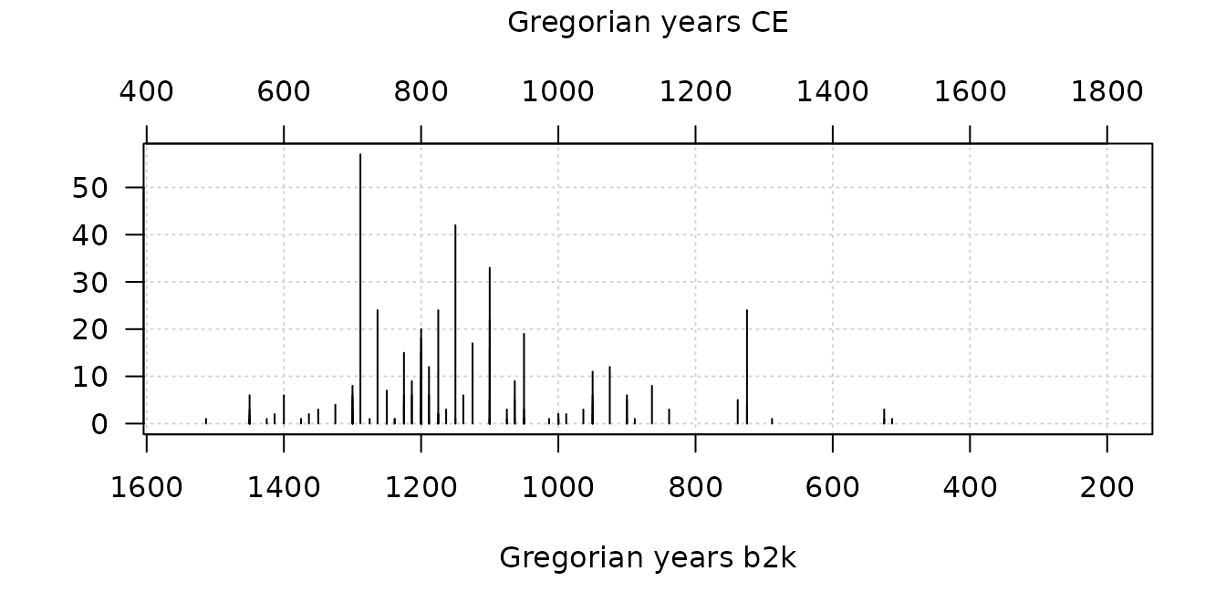
Note that aion uses the astronomical notation for Gregorian years (there is a year 0).
References
Reingold, Edward M., and Nachum Dershowitz. 2018. Calendrical Calculations: The Ultimate Edition. 4th ed. Cambridge University Press. https://doi.org/10.1017/9781107415058.