Visualize Contributions and cos2

Plots contributions histogram and \(cos^2\) scatterplot.

Usage

viz_contributions(x, ...)

viz_cos2(x, ...)

# S4 method for MultivariateAnalysis
viz_contributions(
  x,
  ...,
  margin = 2,
  axes = 1,
  sort = TRUE,
  decreasing = TRUE,
  limit = 10,
  horiz = FALSE,
  col = "grey90",
  border = "grey10"
)

# S4 method for MultivariateAnalysis
viz_cos2(
  x,
  ...,
  margin = 2,
  axes = c(1, 2),
  active = TRUE,
  sup = TRUE,
  sort = TRUE,
  decreasing = TRUE,
  limit = 10,
  horiz = FALSE,
  col = "grey90",
  border = "grey10"
)

Arguments

x

A CA, MCA or PCA object.

...

Extra parameters to be passed to graphics::barplot().

margin

A length-one numeric vector giving the subscript which the data will be returned: 1 indicates individuals/rows (the default), 2 indicates variables/columns.

axes

A numeric vector giving the dimensions to be plotted.

sort

A logical scalar: should the data be sorted?

decreasing

A logical scalar: should the sort order be decreasing? Only used if sort is TRUE.

limit

An integer specifying the number of top elements to be displayed.

horiz

A logical scalar: should the bars be drawn horizontally with the first at the bottom?

col, border

A character string specifying the bars infilling and border colors.

active

A logical scalar: should the active observations be plotted?

sup

A logical scalar: should the supplementary observations be plotted?

Value

viz_contributions() and viz_cos2() are called for their side-effects: they result in a graphic being displayed. Invisibly return x.

Details

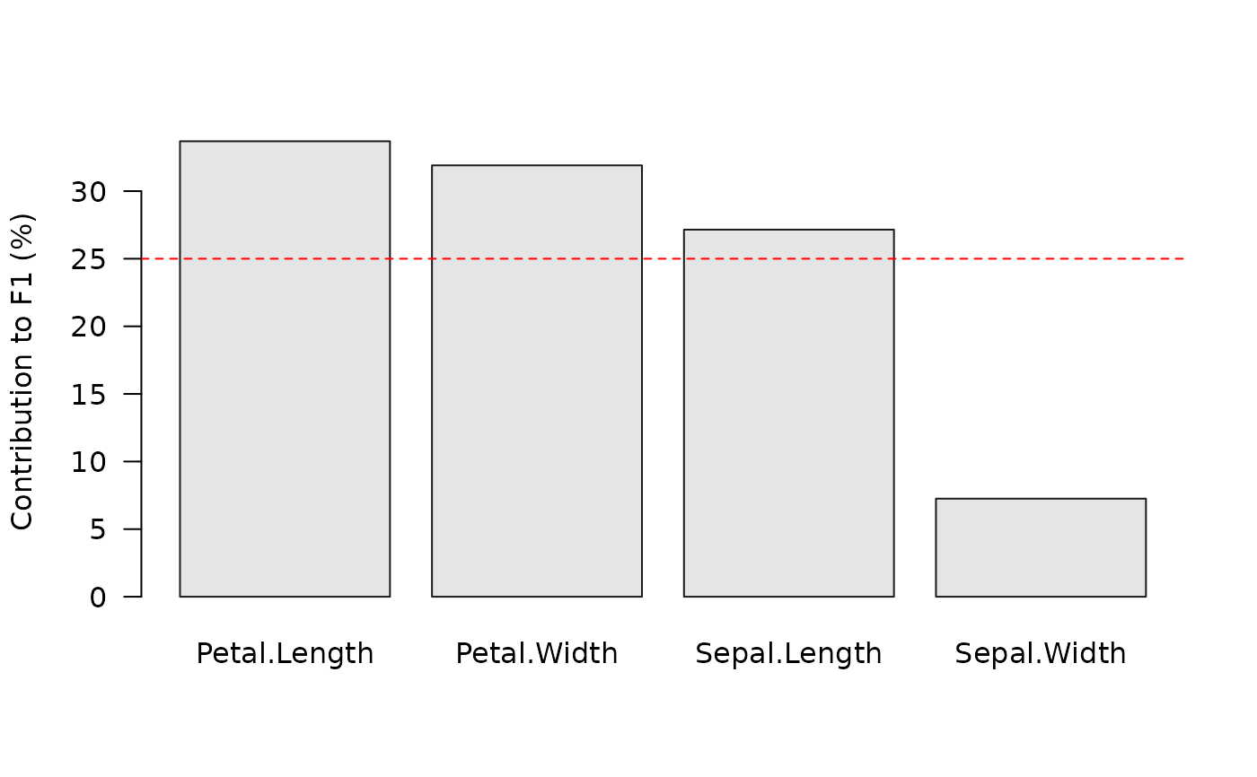
The red dashed line indicates the expected average contribution (variables with a contribution larger than this cutoff can be considered as important in contributing to the component).

See also

Other plot methods: biplot(), screeplot(), viz_individuals(), viz_variables(), viz_wrap, wrap

Author

N. Frerebeau

Examples

## Load data
data("iris")

## Compute principal components analysis
X <- pca(iris, scale = TRUE)
#> 1 qualitative variable was removed: Species.

## Get row contributions
head(get_contributions(X, margin = 1))
#>          F1         F2          F3
#> 1 1.1715796 0.16806554 0.074085470
#> 2 0.9891845 0.33146674 0.250034006
#> 3 1.2768164 0.08526419 0.008875320
#> 4 1.2077372 0.26029781 0.037858004
#> 5 1.3046313 0.30516562 0.001125175
#> 6 0.9841236 1.61748779 0.003303827

## Plot contributions
viz_contributions(X, axes = 1)


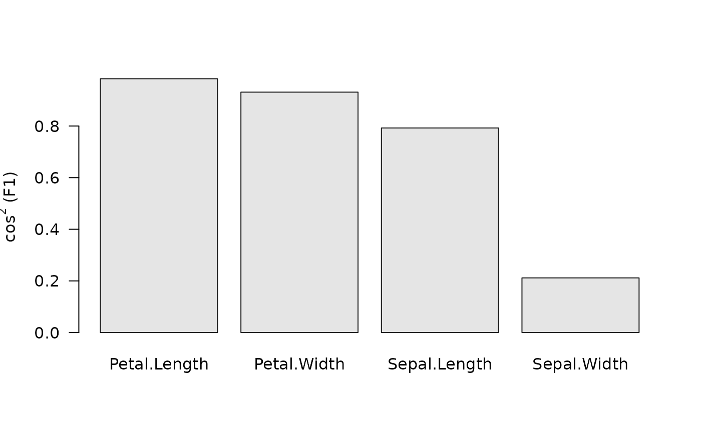
## Plot cos2
viz_cos2(X)