\beta-diversity measures how different local systems are from one another (Moreno and Rodríguez 2010).
tabula allows to calculate several turnover and similarity measures from a count table (absolute frequencies giving the number of individuals for each category, i.e. a contingency table). It assumes that you keep your data tidy: each variable (type/taxa) must be saved in its own column and each observation (sample/case) must be saved in its own row.
## Install extra packages (if needed)
# install.packages("folio") # Datasets

## Load packages
library(tabula)

## Ceramic data from Lipo et al. 2015
data("mississippi", package = "folio")

## Turnover
turnover(mississippi, method = "whittaker")
#> [1] 0.4925373

## Similarity
BR <- similarity(mississippi, method = "brainerd")

## Plot
plot_spot(BR, col = color("YlOrBr")(12))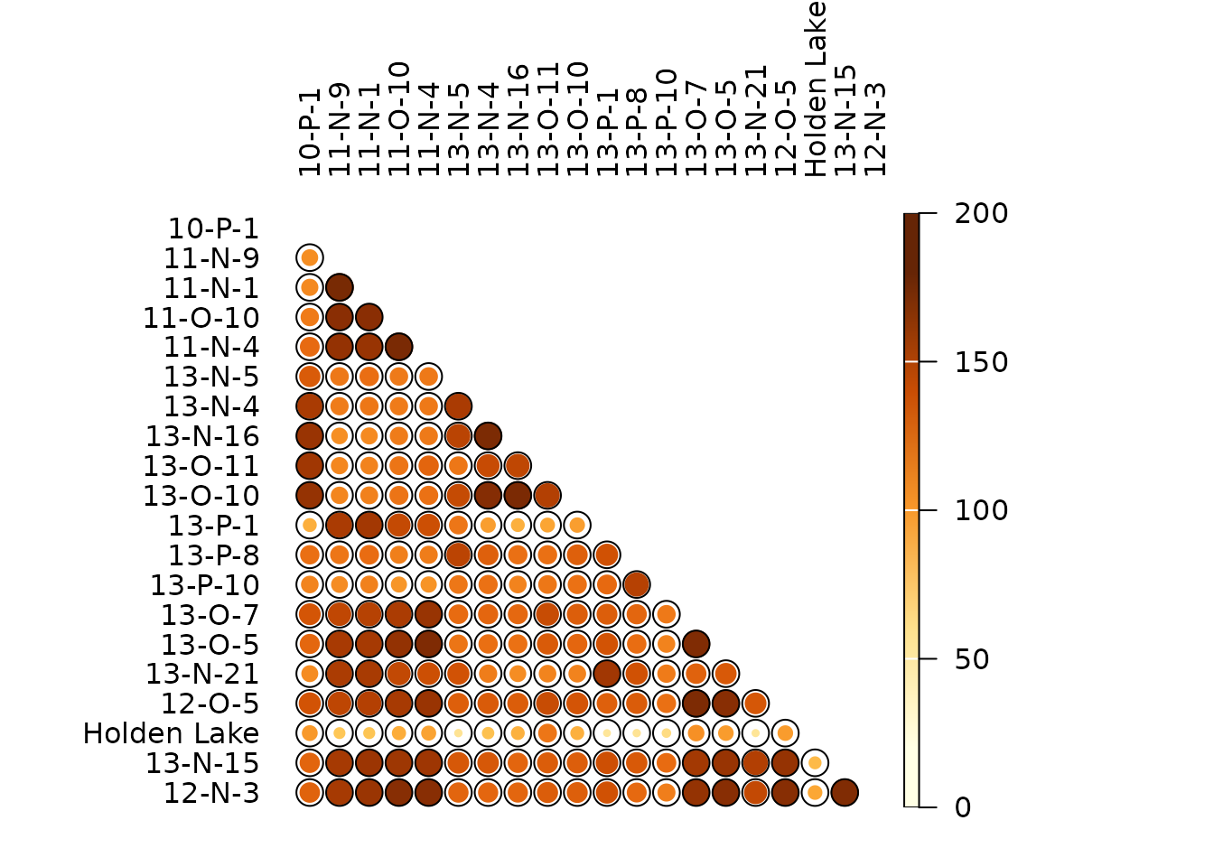
Under the hood, the index_*() functions are called (see
details below).
We denote the m \times p incidence matrix by X = \left[ x_{ij} \right] ~\forall i \in \left[ 1,m \right], j \in \left[ 1,p \right] and the p \times p corresponding co-occurrence matrix by Y = \left[ y_{ij} \right] ~\forall i,j \in \left[ 1,p \right], with row and column sums:
\begin{align} x_{i \cdot} = \sum_{j = 1}^{p} x_{ij} && x_{\cdot j} = \sum_{i = 1}^{m} x_{ij} && x_{\cdot \cdot} = \sum_{j = 1}^{p} \sum_{i = 1}^{m} x_{ij} && \forall x_{ij} \in \lbrace 0,1 \rbrace \\ y_{i \cdot} = \sum_{j \geqslant i}^{p} y_{ij} && y_{\cdot j} = \sum_{i \leqslant j}^{p} y_{ij} && y_{\cdot \cdot} = \sum_{i = 1}^{p} \sum_{j \geqslant i}^{p} y_{ij} && \forall y_{ij} \in \lbrace 0,1 \rbrace \end{align}
## Data from Magurran 1988, p. 162
woodland <- matrix(
  data = c(TRUE, TRUE, TRUE, FALSE, FALSE, FALSE,
           TRUE, TRUE, TRUE, TRUE, TRUE, TRUE,
           FALSE, FALSE, TRUE, FALSE, TRUE, FALSE,
           FALSE, FALSE, FALSE, TRUE, TRUE, TRUE,
           FALSE, FALSE, FALSE, FALSE, TRUE, TRUE,
           FALSE, FALSE, FALSE, TRUE, FALSE, TRUE),
  nrow = 6, ncol = 6
)
colnames(woodland) <- c("Birch", "Oak", "Rowan", "Beech", "Hazel", "Holly")
Turnover
The following methods can be used to ascertain the degree of turnover in taxa composition along a gradient on qualitative (presence/absence) data. This assumes that the order of the matrix rows (from 1 to m) follows the progression along the gradient/transect.
Data are standardized on a presence/absence scale (0/1) beforehand.
Whittaker (1960)
\beta_W = \frac{S}{\alpha} - 1
index_whittaker(woodland)
#> [1] 1
Where \alpha is the mean sample diversity: \alpha = \frac{x_{\cdot \cdot}}{m}
Cody (1975)
\beta_C = \frac{g(H) + l(H)}{2} - 1
Where:
- g(H) is the number of taxa gained along the transect,
- l(H) is the number of taxa lost along the transect.
index_cody(woodland)
#> [1] 3
Routledge 1
\beta_R = \frac{S^2}{2 y_{\cdot \cdot} + S} - 1
index_routledge1(woodland)
#> [1] 0.2857143
Routledge 2
\beta_I = \log x_{\cdot \cdot} - \frac{\sum_{j = 1}^{p} x_{\cdot j} \log x_{\cdot j}}{x_{\cdot \cdot}} - \frac{\sum_{i = 1}^{m} x_{i \cdot} \log x_{i \cdot}}{x_{\cdot \cdot}}
index_routledge2(woodland)
#> [1] 0.5594978Similarity
Similarity between two samples a and b can be measured as follow.
These indices provide a scale of similarity from 0-1 where 1 is perfect similarity and 0 is no similarity, with the exception of the Brainerd-Robinson index which is scaled between 0 and 200.
Thereafter, we denote by:
- S_a and S_b the total number of taxa observed in samples a and b, respectively,
- N_a and N_b the total number of individuals in samples a and b, respectively,
- a_j and b_j the number of individuals in the j-th type/taxon, j \in \left[ 1,S \right],
- o_j the number of type/taxon common to both sample/case: o_j = \sum_{k = 1}^{S} a_k \cap b_k.
Quantitative similarity measures
Brainerd (1951) - Robinson (1951)
C_{BR} = 200 - \sum_{j = 1}^{S} \left| \frac{a_j \times 100}{\sum_{j = 1}^{S} a_j} - \frac{b_j \times 100}{\sum_{j = 1}^{S} b_j} \right|
References
Brainerd, G. W. 1951. The Place of Chronological Ordering in Archaeological Analysis. American Antiquity, 16(4), 301-313. DOI: 10.2307/276979.
Bray, J. R. & Curtis, J. T. (1957). An Ordination of the Upland Forest Communities of Southern Wisconsin. Ecological Monographs, 27(4), 325-349. DOI: 10.2307/1942268.
Cody, M. L. (1975). Towards a Theory of Continental Species Diversity: Bird Distributions Over Mediterranean Habitat Gradients. In M. L. Cody & J. M. Diamond (Eds.), Ecology and Evolution of Communities, 214-257. Cambridge, MA: Harvard University Press.
Dice, L. R. (1945). Measures of the Amount of Ecologic Association Between Species. Ecology, 26(3): 297-302. DOI: 10.2307/1932409.
Horn, H. S. (1966). Measurement of “Overlap” in Comparative Ecological Studies. The American Naturalist, 100(914): 419-424. DOI: 10.1086/282436.
Moreno, C. E. & Rodríguez, P. (2010). A Consistent Terminology for Quantifying Species Diversity? Oecologia, 163(2), 279-782. DOI: 10.1007/s00442-010-1591-7.
Mosrisita, M. (1959). Measuring of interspecific association and similarity between communities. Memoirs of the Faculty of Science, Kyushu University, Series E, 3:65-80.
Robinson, W. S. (1951). A Method for Chronologically Ordering Archaeological Deposits. American Antiquity, 16(4), 293-301. DOI: 10.2307/276978.
Routledge, R. D. (1977). On Whittaker’s Components of Diversity. Ecology, 58(5), 1120-1127. DOI: 10.2307/1936932.
Sorensen, T. (1948). A Method of Establishing Groups of Equal Amplitude in Plant Sociology Based on Similarity of Species Content and Its Application to Analyses of the Vegetation on Danish Commons. Kongelige Danske Videnskabernes Selskab, 5(4): 1-34.
Whittaker, R. H. (1960). Vegetation of the Siskiyou Mountains, Oregon and California. Ecological Monographs, 30(3), 279-338. DOI: 10.2307/1943563..
Wilson, M. V. & Shmida, A. (1984). Measuring Beta Diversity with Presence-Absence Data. The Journal of Ecology, 72(3), 1055-1064. DOI: 10.2307/2259551.