Rarefaction

Rarefaction

Usage

rarefaction(object, ...)

# S4 method for class 'matrix'
rarefaction(object, sample = NULL, method = c("hurlbert", "baxter"), step = 1)

# S4 method for class 'data.frame'
rarefaction(object, sample = NULL, method = c("hurlbert", "baxter"), step = 1)

Arguments

object

A \(m \times p\) numeric matrix or data.frame of count data (absolute frequencies giving the number of individuals for each category, i.e. a contingency table). A data.frame will be coerced to a numeric matrix via data.matrix().

...

Currently not used.

sample

A length-one numeric vector giving the sub-sample size. The size of sample should be smaller than total community size.

method

A character string or vector of strings specifying the index to be computed (see details). Any unambiguous substring can be given.

step

An integer giving the increment of the sample size.

Value

A RarefactionIndex object.

Rarefaction Measures

The following rarefaction measures are available for count data:

baxter

Baxter's rarefaction.

hurlbert

Hurlbert's unbiased estimate of Sander's rarefaction.

Details

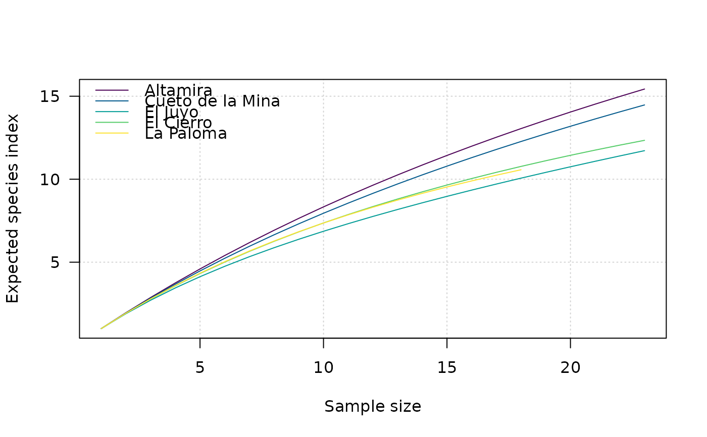
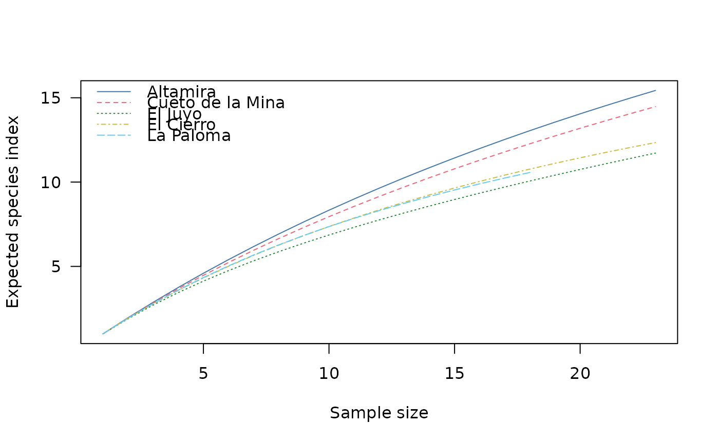
The number of different taxa, provides an instantly comprehensible expression of diversity. While the number of taxa within a sample is easy to ascertain, as a term, it makes little sense: some taxa may not have been seen, or there may not be a fixed number of taxa (e.g. in an open system; Peet 1974). As an alternative, richness (\(S\)) can be used for the concept of taxa number (McIntosh 1967).

It is not always possible to ensure that all sample sizes are equal and the number of different taxa increases with sample size and sampling effort (Magurran 1988). Then, rarefaction (\(E(S)\)) is the number of taxa expected if all samples were of a standard size (i.e. taxa per fixed number of individuals). Rarefaction assumes that imbalances between taxa are due to sampling and not to differences in actual abundances.

See also

index_baxter(), index_hurlbert(), plot()

Other diversity measures: heterogeneity(), occurrence(), plot_diversity, plot_rarefaction, profiles(), richness(), she(), similarity(), simulate(), turnover()

Author

N. Frerebeau

Examples

## Data from Conkey 1980, Kintigh 1989
data("cantabria")

## Replicate fig. 3 from Baxter 2011
rare <- rarefaction(cantabria, sample = 23, method = "baxter")
plot(rare, panel.first = graphics::grid())


## Change graphical parameters
col <- khroma::color("bright")(5)
plot(rare, col = col, lty = 1:5)