Color Schemes
khroma provides an implementation of Okabe (2008), Tol (2021) and Crameri (2018) color schemes for use with base R graphics or ggplot2 and ggraph. These schemes are ready for each type of data (qualitative, diverging or sequential), ready for each type of data, with colors that are:
- Distinct for all people, including color-blind readers,
- Distinct from black and white,
- Distinct on screen and paper,
- Matching well together,
- Citable and reproducible.
See vignette("tol") and vignette("crameri")
for a more complete overview.
For specific uses, several scientific thematic schemes (geologic timescale, land cover, FAO soils, etc.) are implemented, but these color schemes may not be color-blind safe.
The color() function returns a function that when called
with a single integer argument returns a vector of colors:
## Paul Tol's bright color scheme
bright <- color("bright")

## Get seven colors
bright(7)
#> [1] "#4477AA" "#EE6677" "#228833" "#CCBB44" "#66CCEE" "#AA3377" "#BBBBBB"
#> attr(,"missing")
#> [1] NA
Palettes
Discrete Scales
The palette_color_discrete() function allows to map
categorical values to colors. It returns palette function that when
called with a single argument (a vector of categorical values) returns a
character vector of colors:
## Associate each species with a color
bright <- c(versicolor = "#4477AA", virginica = "#EE6677", setosa = "#228833")

## Build a palette function
pal_color <- palette_color_discrete(bright)

## Plot
plot(
  x = iris$Petal.Length,
  y = iris$Sepal.Length,
  col = pal_color(iris$Species), # Map species to colors
  pch = 16,
  xlab = "Petal length",
  ylab = "Sepal length",
  panel.first = grid(),
  las = 1
)
legend("topleft", legend = names(bright), col = bright, pch = 16)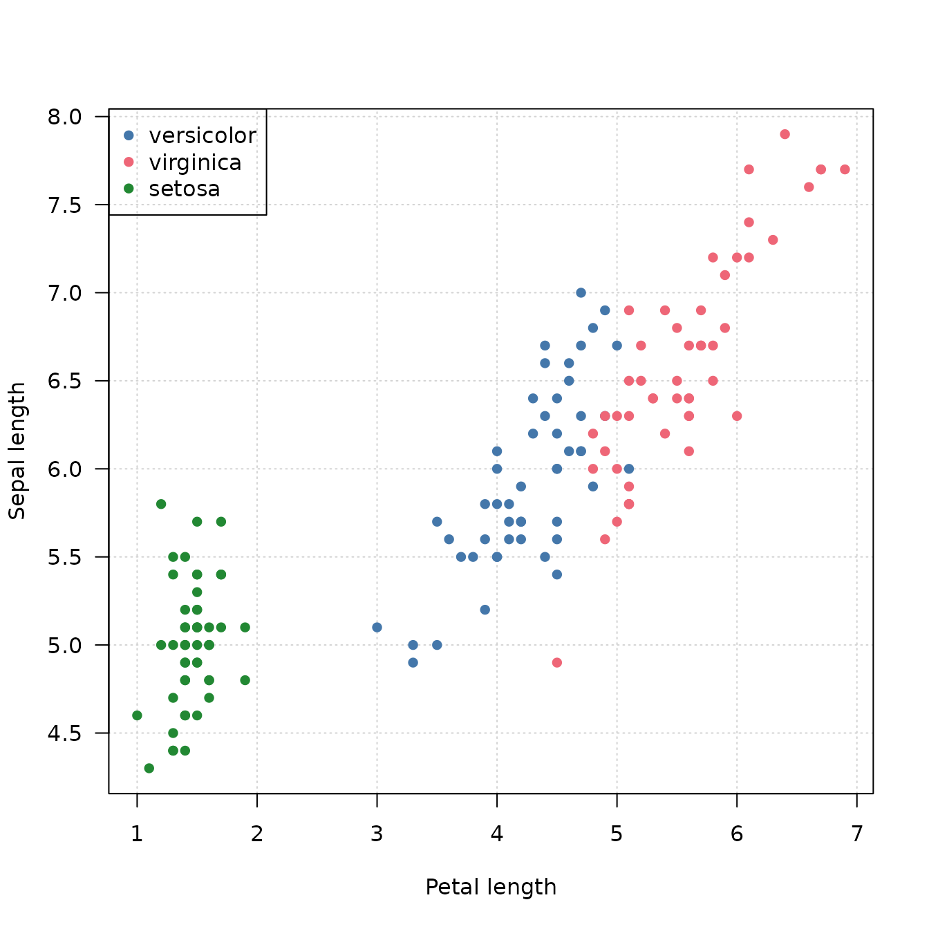
It can be used to highlight a particular level:
## Associate only one species with a color
bright <- c(versicolor = "#4477AA")

## Build a palette function
pal_color <- palette_color_discrete(bright)

## Plot
plot(
  x = iris$Petal.Length,
  y = iris$Sepal.Length,
  col = pal_color(iris$Species),
  pch = 16,
  xlab = "Petal length",
  ylab = "Sepal length",
  panel.first = grid(),
  las = 1
)
legend("topleft", legend = names(bright), col = bright, pch = 16)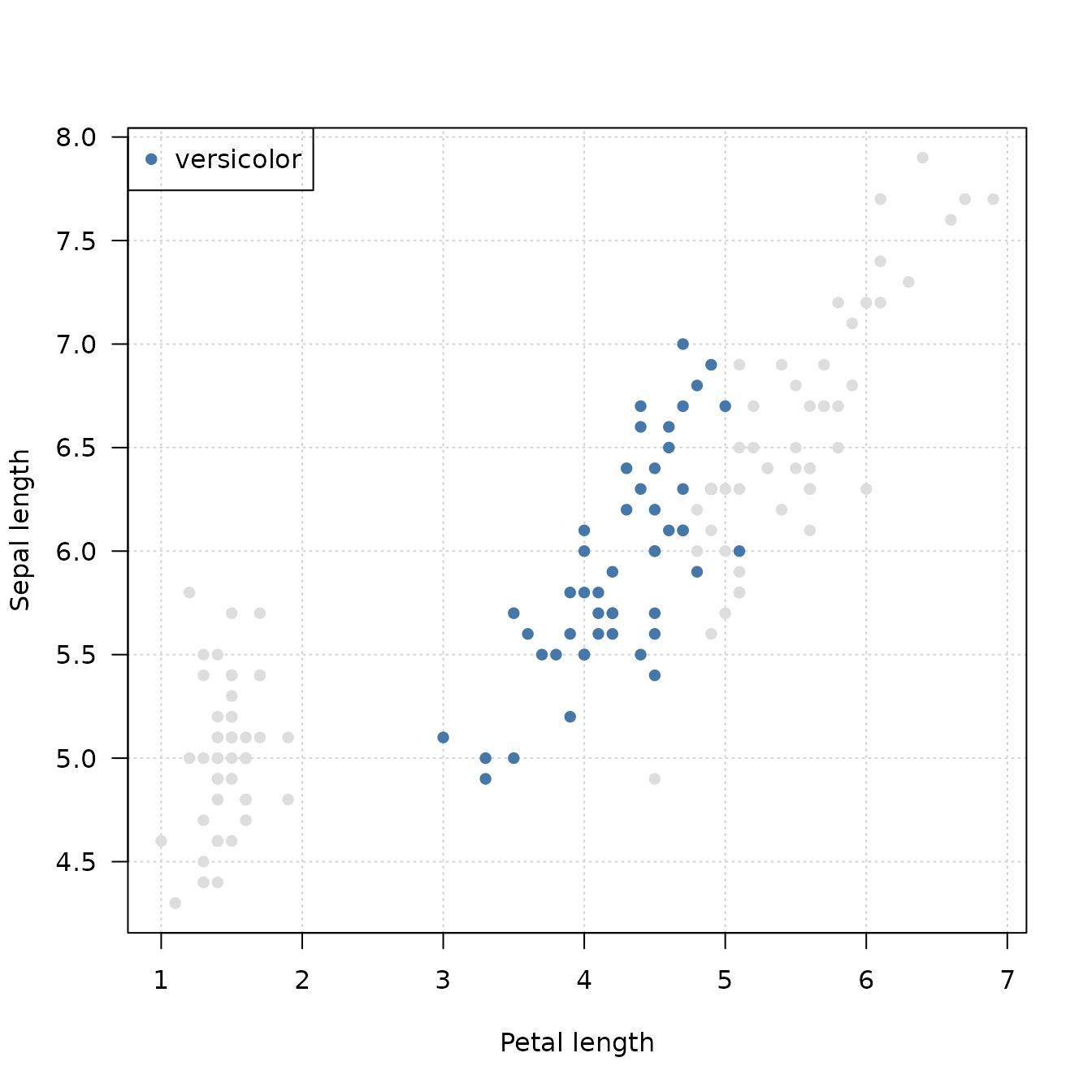
Similarly, the palette_shape() function can be used for
symbol mapping:
## Associate each species with a color
bright <- c(versicolor = "#4477AA", virginica = "#EE6677", setosa = "#228833")
pal_color <- palette_color_discrete(colors = bright)

## Associate each species with a symbol
symbols <- c(versicolor = 15, virginica = 16, setosa = 17)
pal_shapes <- palette_shape(symbols)

## Plot
plot(
  x = iris$Petal.Length,
  y = iris$Sepal.Length,
  col = pal_color(iris$Species), # Map species to colors
  pch = pal_shapes(iris$Species), # Map species to symbols
  xlab = "Petal length",
  ylab = "Sepal length",
  panel.first = grid(),
  las = 1
)
legend("topleft", legend = names(bright), col = bright, pch = symbols)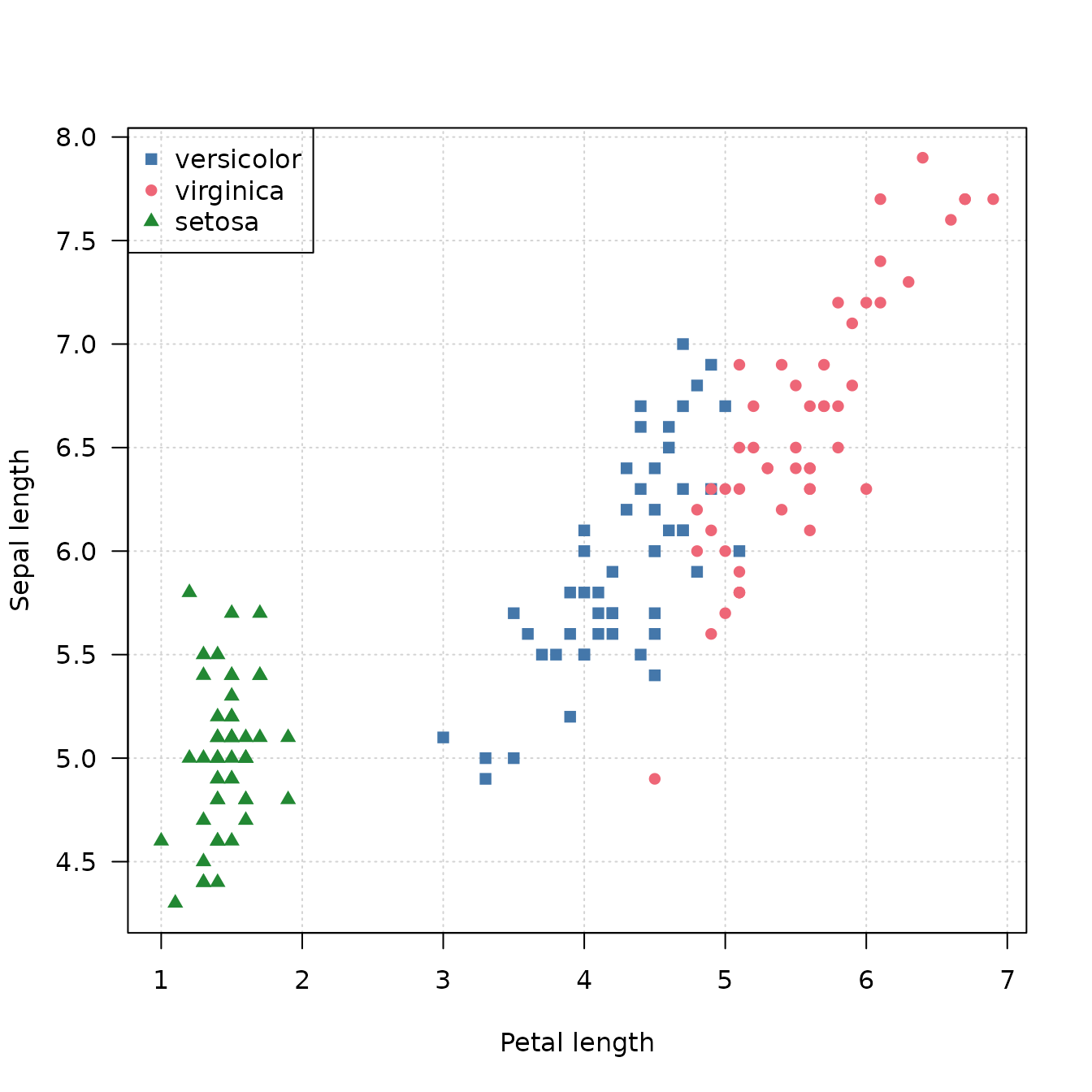
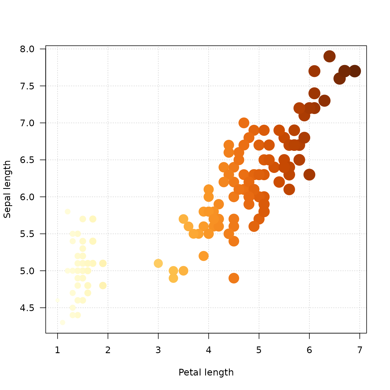
Continuous Scales
The palette_color_continuous() and
palette_size_sequential() functions can be used to map
continuous values to colors and symbol sizes:
## Scatter plot
## Build a color palette function
YlOrBr <- color("YlOrBr")
pal_color <- palette_color_continuous(colors = YlOrBr)

## Build a symbol palette function
pal_size <- palette_size_sequential(range = c(1, 3))

## Plot
plot(
  x = iris$Petal.Length,
  y = iris$Sepal.Length,
  pch = 16,
  col = pal_color(iris$Petal.Length),
  cex = pal_size(iris$Petal.Length),
  xlab = "Petal length",
  ylab = "Sepal length",
  panel.first = grid(),
  las = 1
)
References
Crameri, Fabio. 2018. Geodynamic Diagnostics, Scientific Visualisation and StagLab 3.0. Geoscientific Model Development 11 (6): 2541–62. https://doi.org/10.5194/gmd-11-2541-2018.
Okabe, Masataka, and Key Ito. 2008. Color Universal Design (CUD): How to Make Figures and Presentations That Are Friendly to Colorblind People. J*FLY. https://jfly.uni-koeln.de/color/.
Tol, Paul. 2021. Colour Schemes. Technical note SRON/EPS/TN/09-002 3.2. SRON. https://sronpersonalpages.nl/~pault/data/colourschemes.pdf.