Histogram of Compositional Data

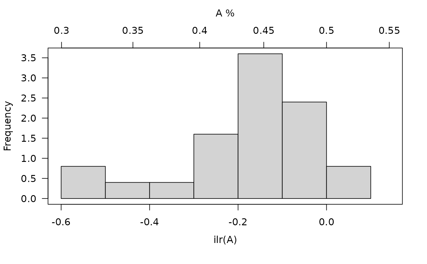
Produces an histogram of univariate ILR data (see Filzmoser et al., 2009).

Usage

# S4 method for class 'CompositionMatrix'
hist(
  x,
  ...,
  select = 1,
  breaks = "Sturges",
  freq = FALSE,
  labels = FALSE,
  main = NULL,
  sub = NULL,
  ann = graphics::par("ann"),
  axes = TRUE,
  frame.plot = axes
)

Arguments

x

A CompositionMatrix object.

...

Further graphical parameters.

select

A length-one vector of column indices.

breaks

An object specifying how to compute the breakpoints (see graphics::hist()).

freq

A logical scalar: should absolute frequencies (counts) be displayed? If FALSE (the default), relative frequencies (probabilities) are displayed (see graphics::hist()).

labels

A logical scalar: should labels be drawn on top of bars? If TRUE, draw the counts or rounded densities; if labels is a character vector, draw itself.

main

A character string giving a main title for the plot.

sub

A character string giving a subtitle for the plot.

ann

A logical scalar: should the default annotation (title and x and y axis labels) appear on the plot?

axes

A logical scalar: should axes be drawn on the plot?

frame.plot

A logical scalar: should a box be drawn around the plot?

Value

hist() is called for its side-effects: is results in a graphic being displayed (invisibly return x).

References

Filzmoser, P., Hron, K. & Reimann, C. (2009). Univariate Statistical Analysis of Environmental (Compositional) Data: Problems and Possibilities. Science of The Total Environment, 407(23): 6100-6108. doi:10.1016/j.scitotenv.2009.08.008 .

See also

Other plot methods: as_graph(), barplot(), pairs(), plot()

Author

N. Frerebeau

Examples

## Data from Aitchison 1986
data("hongite")

## Coerce to compositional data
coda <- as_composition(hongite)

## Boxplot plot
hist(coda, select = "A")

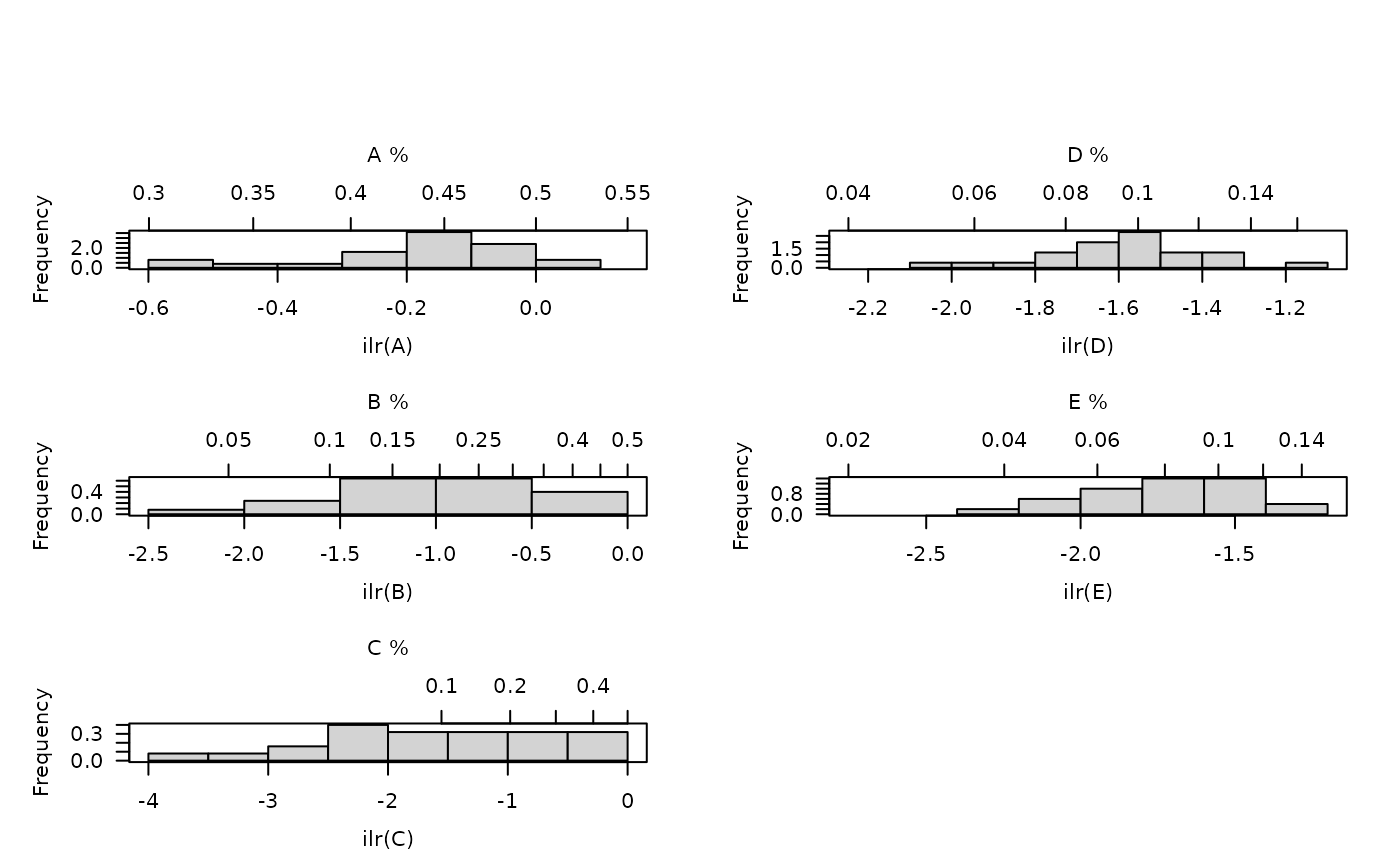hist(coda, select = "B")