## Install extra packages (if needed)
# install.packages("folio") # datasets

library(nexus)
#> Loading required package: dimensio
Reference Groups
Provenance studies typically rely on two approaches, which can be used together:
- Identification of groups among the artifacts being studied, based on mineralogical or geochemical criteria (clustering).
- Comparison with so-called reference groups, i.e. known geological sources or archaeological contexts (classification).
We use here the results of the analysis of 369 ancient bronzes (see
help(bronze, package = "folio")) attributed to three
dynasties. For the sake of the demonstration, let’s assume that a third
of the samples are of unknown provenance: missing values
(NA) can be used to specify that a sample does not belong
to any group.
## Data from Wood and Liu 2023
data("bronze", package = "folio")
dynasty <- as.character(bronze$dynasty) # Save original data for further use

## Randomly add missing values
set.seed(12345) # Set seed for reproductibility
n <- nrow(bronze)
bronze$dynasty[sample(n, size = n / 3)] <- NA
When coercing a data.frame to a
CompositionMatrix object, nexus allows to
specify whether an observation belongs to a specific group (or not):
## Use the third column (dynasties) for grouping
coda <- as_composition(bronze, parts = 4:11, groups = 3)
Alternatively, group() allows to set groups of an
existing CompositionMatrix.
## Create a composition data matrix
coda <- as_composition(bronze, parts = 4:11)

## Use the third dynasties for grouping
coda <- group(coda, by = bronze$dynasty)
Once groups have been defined, they can be used by further methods (e.g. plotting). Note that for better readability, you can select only some of the parts (e.g. major elements):
## Select major elements
major <- coda[, is_element_major(coda)]

## Compositional bar plot
barplot(major, order_rows = "Cu", space = 0)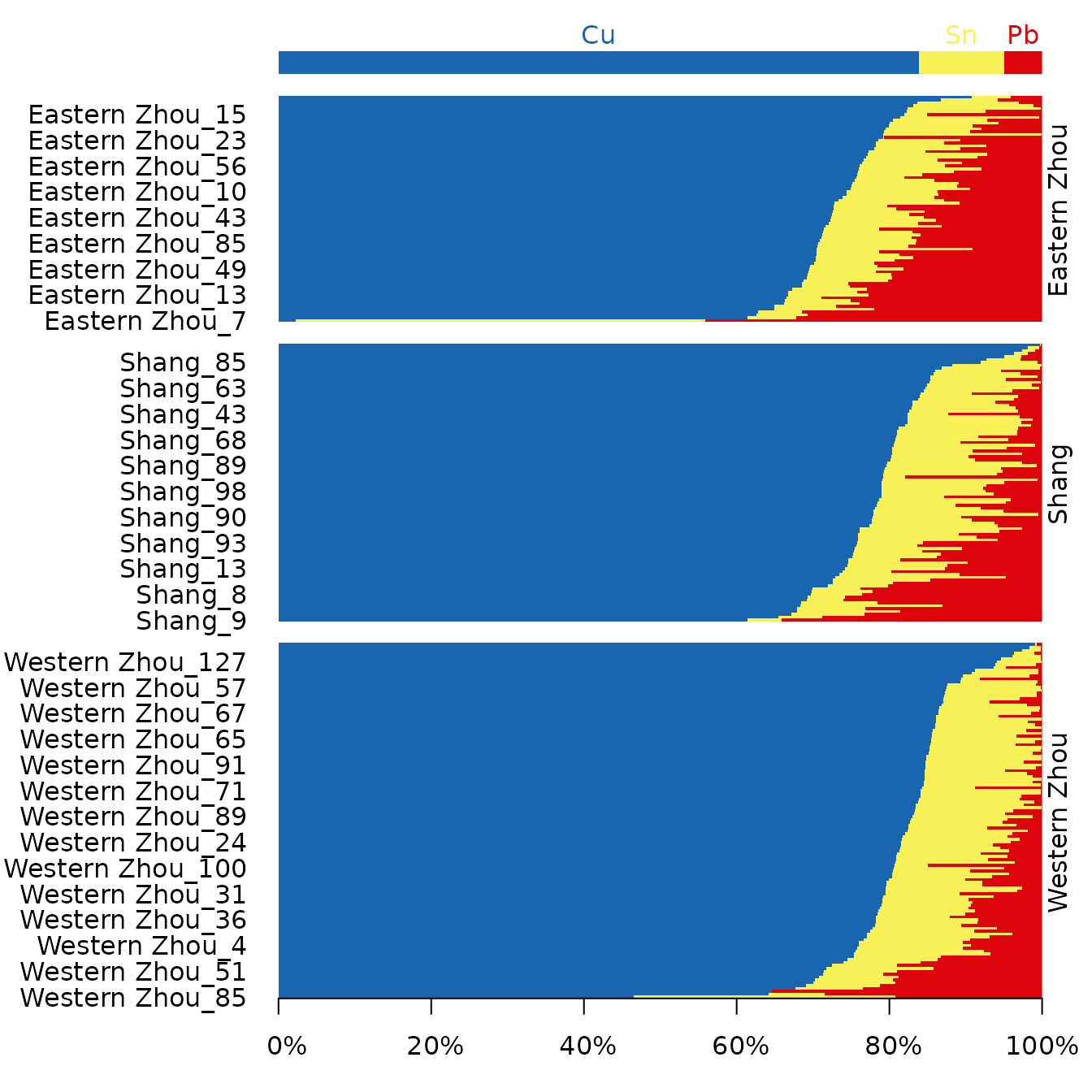
## Matrix of ternary plots
pairs(coda)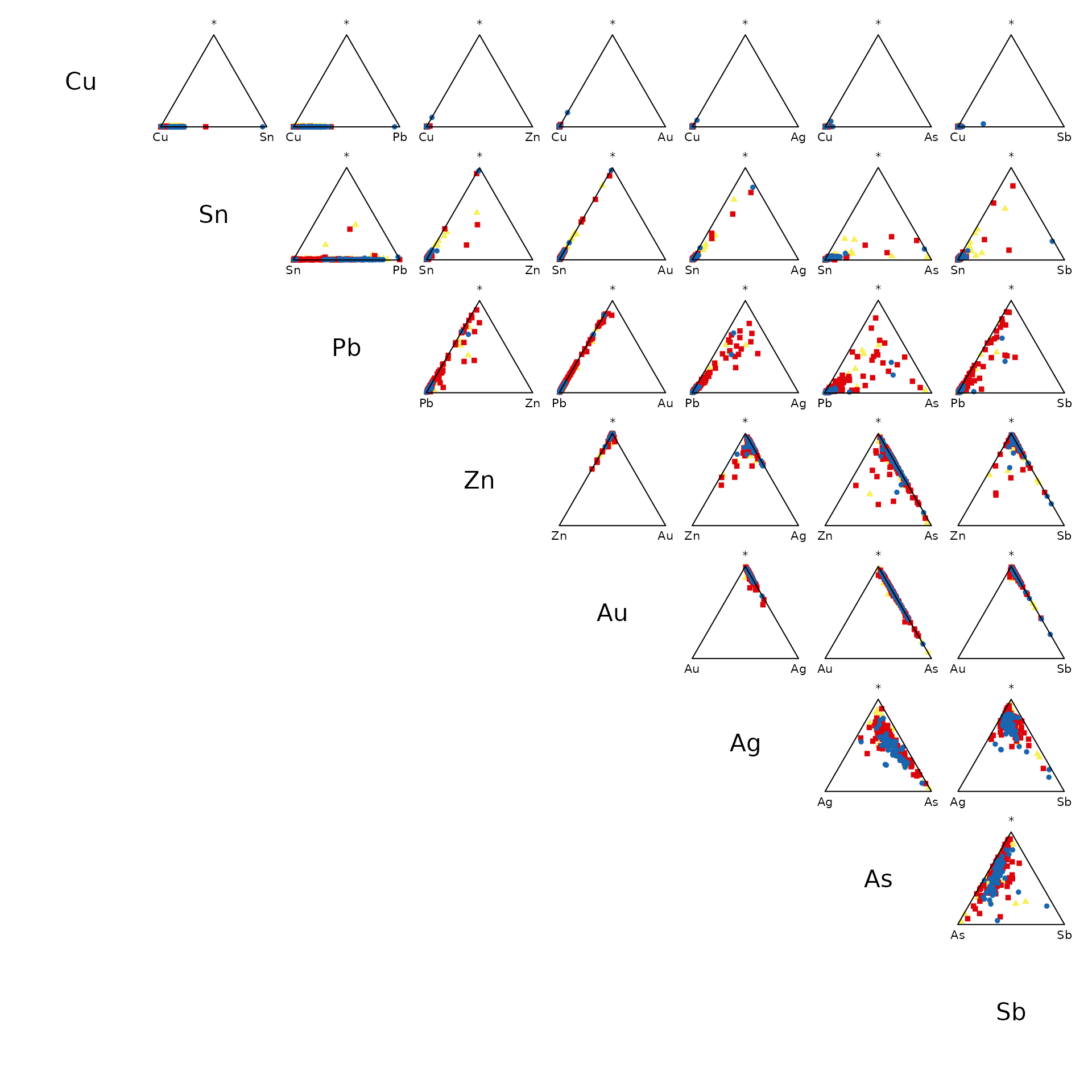
Log-Ratio Analysis
## CLR
clr <- transform_clr(coda, weights = TRUE)

## PCA
lra <- pca(clr)

## Visualize results
viz_individuals(
  x = lra,
  extra_quali = group_names(clr),
  color = c("#004488", "#DDAA33", "#BB5566"),
  hull = TRUE
)

viz_variables(lra)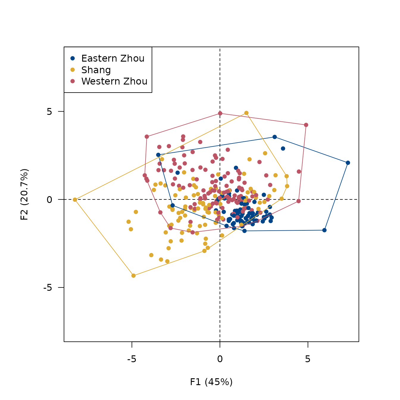

Discriminant Analysis
## Subset training data
train <- coda[is_assigned(coda), ]

## ILR
ilr_train <- transform_ilr(train)

## MANOVA
fit <- manova(ilr_train ~ group_names(ilr_train))
summary(fit)
#>                         Df  Pillai approx F num Df den Df    Pr(>F)
#> group_names(ilr_train)   2 0.48784   10.969     14    476 < 2.2e-16 ***
#> Residuals              243
#> ---
#> Signif. codes:  0 '***' 0.001 '**' 0.01 '*' 0.05 '.' 0.1 ' ' 1
The MANOVA results suggest that there are statistically significant differences between groups.
Let’s now try how effective a Linear Discriminant Analysis (LDA) is at separating the three groups:
## LDA
(discr <- MASS::lda(ilr_train, grouping = group_names(ilr_train)))
#> Call:
#> lda(ilr_train, grouping = group_names(ilr_train))
#>
#> Prior probabilities of groups:
#> Eastern Zhou        Shang Western Zhou
#>    0.2886179    0.2520325    0.4593496
#>
#> Group means:
#>                     Z1         Z2        Z3        Z4        Z5         Z6
#> Eastern Zhou -1.364512 -0.5482067 -7.299353 -6.189647 -1.480905 -0.2409364
#> Shang        -1.513779 -1.4812935 -6.474733 -6.755594 -1.972246 -0.7178804
#> Western Zhou -1.419500 -2.0435454 -6.326308 -6.027864 -1.860501 -0.5915081
#>                     Z7
#> Eastern Zhou -1.438962
#> Shang        -2.415992
#> Western Zhou -1.964109
#>
#> Coefficients of linear discriminants:
#>            LD1        LD2
#> Z1 -0.39979112  0.7933790
#> Z2 -0.54894961 -0.2738935
#> Z3  0.17240912  0.2650783
#> Z4  0.02471627  0.7357643
#> Z5 -1.15794427  0.1568422
#> Z6 -0.09169188 -0.1163724
#> Z7 -0.02495294  0.7914043
#>
#> Proportion of trace:
#>    LD1    LD2
#> 0.6594 0.3406
By default, some of these results (group averages and discriminant function coefficients) are reported in ILR coordinates, making them difficult to interpret. Therefore, it is preferable to transform these results back into compositions or equivalent CLR coefficients:
## Back transform results
transform_inverse(discr$means, origin = ilr_train)
#>                     Cu         Sn         Pb           Zn           Au
#> Eastern Zhou 0.7414243 0.10764753 0.14435915 4.935810e-05 2.712054e-05
#> Shang        0.8498753 0.09991134 0.04748813 9.013678e-05 1.287939e-05
#> Western Zhou 0.8558980 0.11497046 0.02567689 9.155170e-05 2.595307e-05
#>                        Ag          As           Sb
#> Eastern Zhou 0.0013586267 0.004047536 0.0010863861
#> Shang        0.0006248601 0.001741556 0.0002557903
#> Western Zhou 0.0007422594 0.002141355 0.0004535491
plot(discr, col = c("#DDAA33", "#BB5566", "#004488")[group_indices(ilr_train)])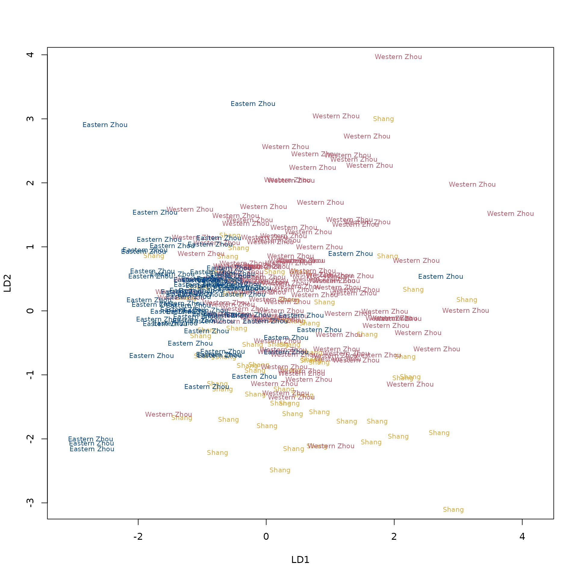
We can then try to predict the group membership of the unassigned samples:
## Subset unassigned samples
test <- coda[!is_assigned(coda), ]
ilr_test <- transform_ilr(test)

## Predict group membership
results <- predict(discr, ilr_test)

## Assess the accuracy of the prediction
(ct <- table(
  predicted = results$class,
  expected = dynasty[!is_assigned(coda)]
))
#>               expected
#> predicted      Eastern Zhou Shang Western Zhou
#>   Eastern Zhou           19     8            8
#>   Shang                   0    28            8
#>   Western Zhou            8    13           31
diag(proportions(ct, margin = 1))
#> Eastern Zhou        Shang Western Zhou
#>    0.5428571    0.7777778    0.5961538

## Total percent correct
sum(diag(proportions(ct)))
#> [1] 0.6341463