Provenance studies rely on the identification of probable sources, such that the variability between two sources is greater than the internal variability of a single source (the so-called provenance postulate; Weigand, Harbottle, and Sayre 1977). This assumes that a unique signature can be identified for each source on the basis of several criteria.
nexus is designed for chemical fingerprinting and source tracking of ancient materials. It provides provides tools for exploration and analysis of compositional data in the framework of Aitchison (1986). If you are unfamiliar with the concepts and challenges of compositional data analysis, the following publications are a good place to start:
- Egozcue, J. J., Gozzi, C., Buccianti, A. & Pawlowsky-Glahn, V. (2024). Exploring Geochemical Data Using Compositional Techniques: A Practical Guide. Journal of Geochemical Exploration, 258: 107385. DOI: 10.1016/j.gexplo.2024.107385.
- Greenacre, M. & Wood, J. R. (2024). A Comprehensive Workflow for Compositional Data Analysis in Archaeometry, with Code in R. Archaeological and Anthropological Science, 16: 171. DOI: 10.1007/s12520-024-02070-w
- Grunsky, E., Greenacre, M. & Kjarsgaard, B. (2024). GeoCoDA: Recognizing and Validating Structural Processes in Geochemical Data. A Workflow on Compositional Data Analysis in Lithogeochemistry. Applied Computing and Geosciences, 22: 100149. DOI: 10.1016/j.acags.2023.100149.
Get started
## Install extra packages (if needed)
# install.packages("folio") # datasets
# install.packages("isopleuros") # ternary plot

library(nexus)
nexus provides a set of S4 classes that represent different special types of matrix. The most basic class represents a compositional data matrix, i.e. quantitative (positive) descriptions of the parts of some whole, carrying relative, rather than absolute, information (Aitchison 1986; Greenacre 2019).
It assumes that you keep your data tidy: each variable must be saved in its own column and each observation (sample) must be saved in its own row.
This class is of simple use as it inherits from base
matrix:
## Mineral compositions of rock specimens
## Data from Aitchison 1986
data("hongite")
head(hongite)
#>       A    B    C    D    E
#> H1 48.8 31.7  3.8  6.4  9.3
#> H2 48.2 23.8  9.0  9.2  9.8
#> H3 37.0  9.1 34.2  9.5 10.2
#> H4 50.9 23.8  7.2 10.1  8.0
#> H5 44.2 38.3  2.9  7.7  6.9
#> H6 52.3 26.2  4.2 12.5  4.8

## Coerce to compositional data
coda <- as_composition(hongite)
head(coda)
#> <CompositionMatrix: 6 x 5>
#>        A     B     C     D     E
#> H1 0.488 0.317 0.038 0.064 0.093
#> H2 0.482 0.238 0.090 0.092 0.098
#> H3 0.370 0.091 0.342 0.095 0.102
#> H4 0.509 0.238 0.072 0.101 0.080
#> H5 0.442 0.383 0.029 0.077 0.069
#> H6 0.523 0.262 0.042 0.125 0.048
A CompositionMatrix represents a closed
composition matrix: each row of the matrix sum up to 1 (only relative
changes are relevant in compositional data analysis).
The original row sums are kept internally, so that the source data can be restored:
## Coerce to count data
counts <- as_amounts(coda)

all.equal(hongite, as.data.frame(counts))
#> [1] TRUE
The parts argument of the function
as_composition() is used to define the columns to be used
as the compositional part. If parts is NULL
(the default), all numeric columns are used. In the case of
a data.frame coercion, additional columns are removed.
## Create a data.frame
X <- data.frame(
  type = c("A", "A", "B", "A", "B", "C", "C", "C", "B"),
  Ca = c(7.72, 7.32, 3.11, 7.19, 7.41, 5, 4.18, 1, 4.51),
  Fe = c(6.12, 5.88, 5.12, 6.18, 6.02, 7.14, 5.25, 5.28, 5.72),
  Na = c(0.97, 1.59, 1.25, 0.86, 0.76, 0.51, 0.75, 0.52, 0.56)
)

## Coerce to a compositional matrix
## (the 'type' column will be removed)
Y <- as_composition(X)
It is also possible to define a grouping variable (see
vignette("groups")):
## Coerce to a compositional matrix
## (the 'type' column will be used for group definition)
Y <- as_composition(X, group = 1)
Repeated measurements
If your data contain several observations for the same sample (e.g. repeated measurements), you can use one or more categorical variable to split the data into subsets and compute the compositional mean for each:
## Data from Wood and Liu 2023
data("bronze", package = "folio")

## Create a composition data matrix
coda <- as_composition(bronze, parts = 4:11)

## Compositional mean by artefact
coda <- condense(coda, by = list(bronze$dynasty, bronze$reference))
Descriptive statistics
Several compositional statistics can be calculated:
-
covariance(): (centered) log-ratio covariance matrix (Aitchison 1986); -
dist(): Aitchison distance (euclidean distance on CLR-transformed data); -
mean(): compositional mean (Aitchison 1986); -
pip(): proportionality index of parts (Egozcue & Pawlowsky-Glahn 2023); -
quantile(): sample quantiles; -
variation(): variation matrix (Aitchison 1986).
## Compositional mean
mean(coda)
#>           Cu           Sn           Pb           Zn           Au           Ag
#> 8.353725e-01 1.112853e-01 4.976821e-02 7.299130e-05 2.057024e-05 8.358320e-04
#>           As           Sb
#> 2.194956e-03 4.495890e-04
Data visualization
Compositional data are multivariate data for which relative values are important: they can easily be visualized using stacked bar charts showing sample composition.
Note that for better readability, you can select only some of the parts (e.g. major elements), but keep in mind that the percentages displayed may change radically if additional parts are added/deleted (principle of subcompositional coherence; Greenacre 2019).
## Select major elements
major <- coda[, is_element_major(coda)]

## Compositional bar plot
barplot(major, order_rows = "Cu", order_columns = TRUE, space = 0)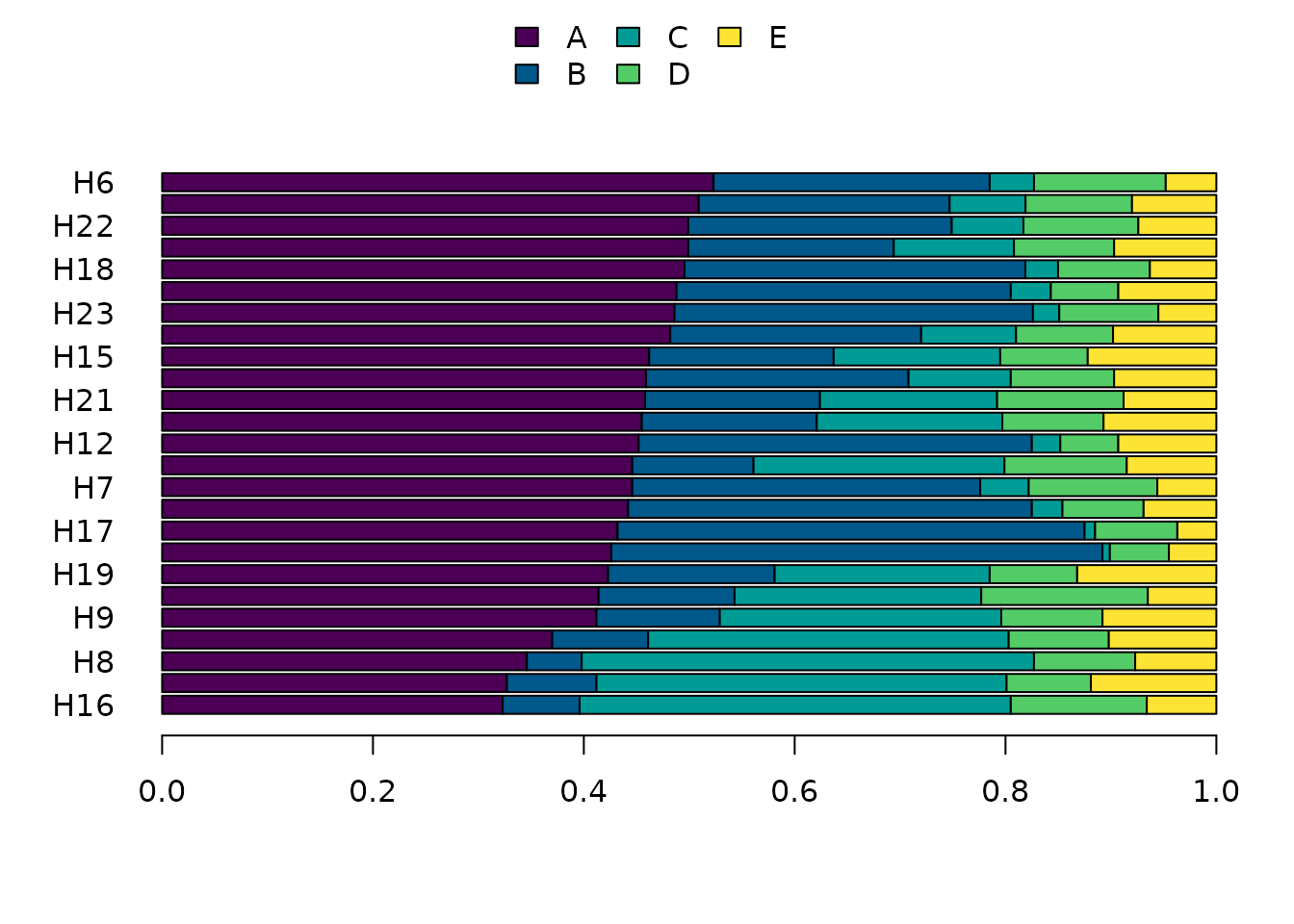
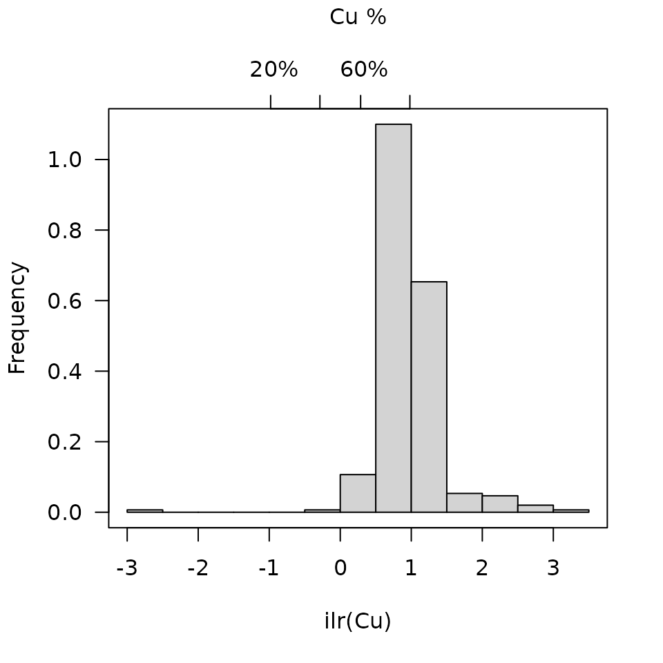
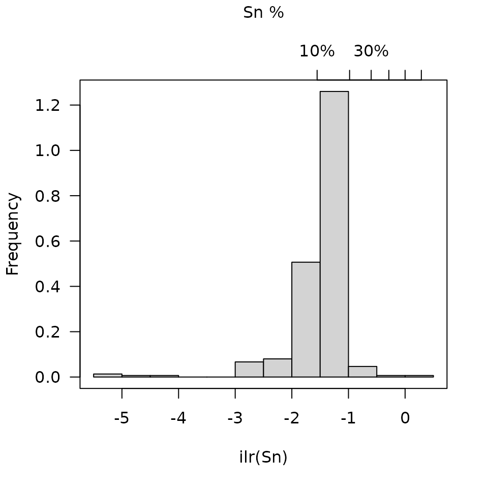
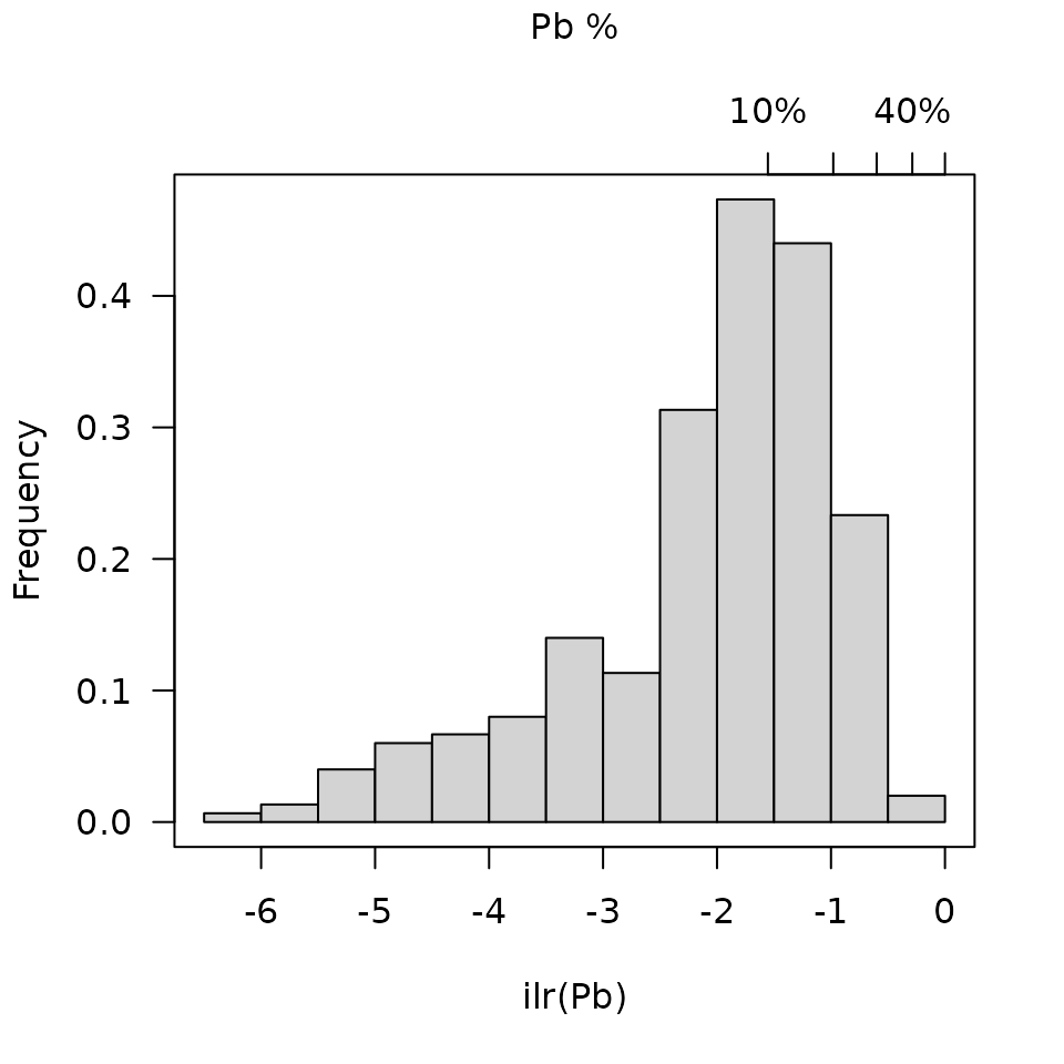
As described by Filzmoser et al. (2009), histograms (showing univariate distributions) can be calculated and plotted:
isopleuros is a companion package to nexus that allows to create ternary plots:
## Load
library(isopleuros)

## Cu-Sn-Pb ternary plot
CuSnPb <- coda[, c("Cu", "Sn", "Pb")]
ternary_plot(CuSnPb)
ternary_grid()
Log-ratio transformations
The package provides the following (inverse) transformations:
-
transform_clr(): centered log ratio (CLR, Aitchison 1986); -
transform_alr(): additive log ratio (ALR, Aitchison 1986); -
transform_ilr(): isometric log ratio (ILR, Egozcue et al. 2003); -
transform_plr(): pivot log-ratio (PLR, Hron et al. 2017).
## CLR
clr <- transform_clr(coda)

## Back transform
back <- transform_inverse(clr)

all.equal(back, coda)
#> [1] TRUE
References
Aitchison, J. (1986). The Statistical Analysis of Compositional Data. Monographs on Statistics and Applied Probability. Londres, UK ; New York, USA: Chapman and Hall.
Egozcue, J. J. and Pawlowsky-Glahn, V. (2023). Subcompositional Coherence and and a Novel Proportionality Index of Parts. SORT, 47(2): 229-244. DOI: 10.57645/20.8080.02.7.
Egozcue, J. J., Pawlowsky-Glahn, V., Mateu-Figueras, G. and Barceló-Vidal, C. (2003). Isometric Logratio Transformations for Compositional Data Analysis. Mathematical Geology, 35(3): 279-300. DOI: 10.1023/A:1023818214614.
Filzmoser, P., Hron, K. and Reimann, C. (2009). Univariate Statistical Analysis of Environmental (Compositional) Data: Problems and Possibilities. Science of The Total Environment, 407(23): 6100-6108. DOI: 10.1016/j.scitotenv.2009.08.008.
Greenacre, M. J. (2019). Compositional Data Analysis in Practice. Chapman & Hall/CRC Interdisciplinary Statistics. Boca Raton: CRC Press, Taylor & Francis Group.
Hron, K., Filzmoser, P., de Caritat, P., Fišerová, E. and Gardlo, A. (2017). Weighted Pivot Coordinates for Compositional Data and Their Application to Geochemical Mapping. Mathematical Geosciences, 49(6): 797-814. DOI : 10.1007/s11004-017-9684-z.
Weigand, P. C., Harbottle, G. and Sayre, E. (1977). Turquoise Sources and Source Analysisis: Mesoamerica and the Southwestern U.S.A. In J. Ericson & T. K. Earle (Eds.), Exchange Systems in Prehistory, 15-34. New York, NY: Academic Press.