Diversity Plot

Diversity Plot

Usage

# S4 method for class 'DiversityIndex,missing'
plot(
  x,
  log = "x",
  col.mean = "#DDAA33",
  col.interval = "#004488",
  lty.mean = "solid",
  lty.interval = "dashed",
  lwd.mean = 1,
  lwd.interval = 1,
  xlab = NULL,
  ylab = NULL,
  main = NULL,
  sub = NULL,
  ann = graphics::par("ann"),
  axes = TRUE,
  frame.plot = axes,
  panel.first = NULL,
  panel.last = NULL,
  ...
)

Arguments

x

A DiversityIndex object to be plotted.

log

A character string indicating which axes should be in log scale. Defaults to x.

col.mean, col.interval

A character string specifying the color of the lines.

lty.mean, lty.interval

A character string or numeric value specifying the line types.

lwd.mean, lwd.interval

A non-negative numeric value specifying the line widths.

xlab, ylab

A character vector giving the x and y axis labels.

main

A character string giving a main title for the plot.

sub

A character string giving a subtitle for the plot.

ann

A logical scalar: should the default annotation (title and x, y and z axis labels) appear on the plot?

axes

A logical scalar: should axes be drawn on the plot?

frame.plot

A logical scalar: should a box be drawn around the plot?

panel.first

An an expression to be evaluated after the plot axes are set up but before any plotting takes place. This can be useful for drawing background grids.

panel.last

An expression to be evaluated after plotting has taken place but before the axes, title and box are added.

...

Further graphical parameters to be passed to graphics::points(), particularly, cex, col and pch.

Value

plot() is called for its side-effects: it results in a graphic being displayed (invisibly returns x).

See also

Other diversity measures: diversity(), evenness(), heterogeneity(), occurrence(), plot.RarefactionIndex(), profiles(), rarefaction(), richness(), she(), similarity(), simulate(), turnover()

Author

N. Frerebeau

Examples

# \donttest{
## Data from Conkey 1980, Kintigh 1989
data("cantabria")

## Assemblage diversity size comparison
## Warning: this may take a few seconds!
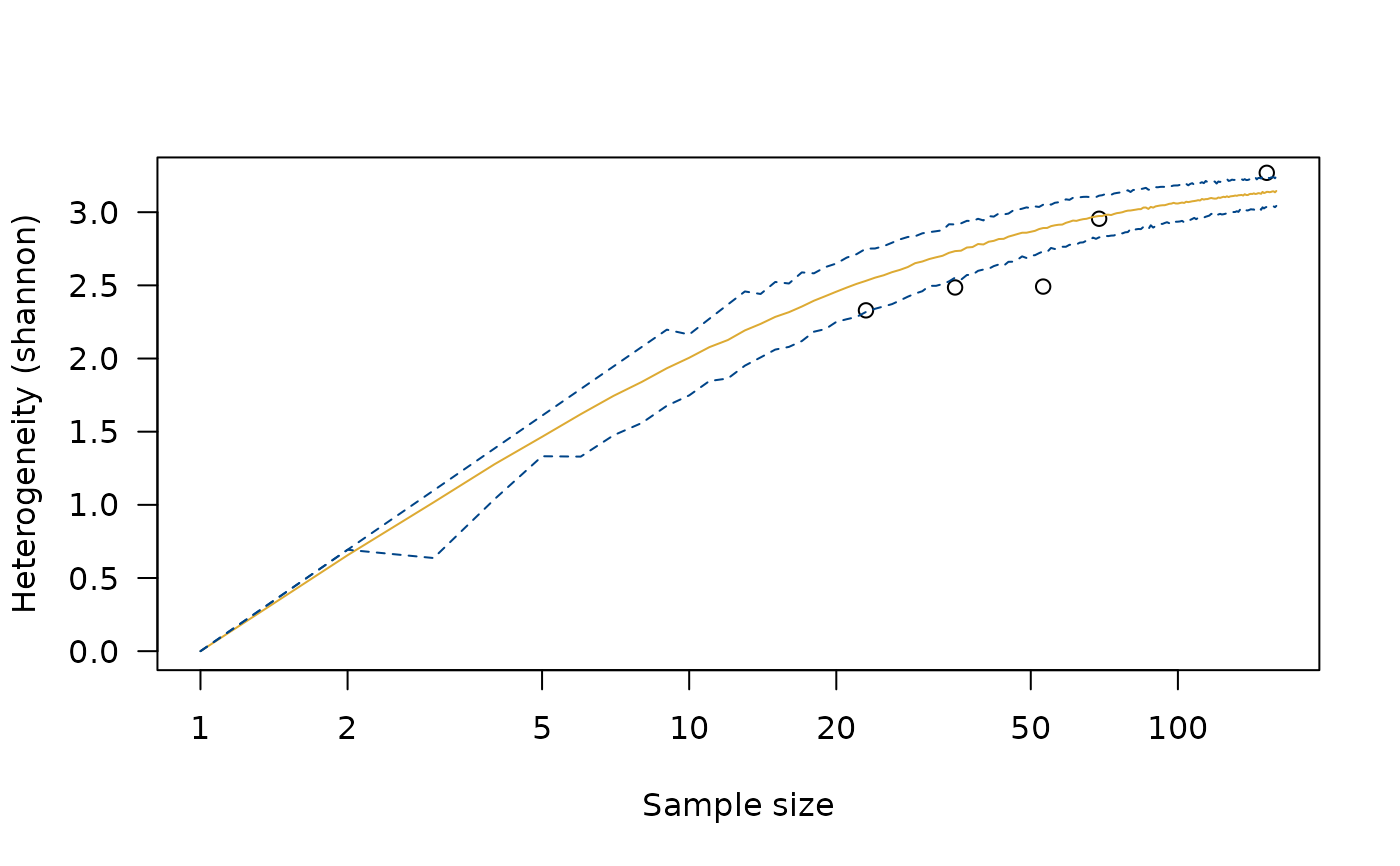
h <- heterogeneity(cantabria, method = "shannon")
h_sim <- simulate(h)
plot(h_sim)


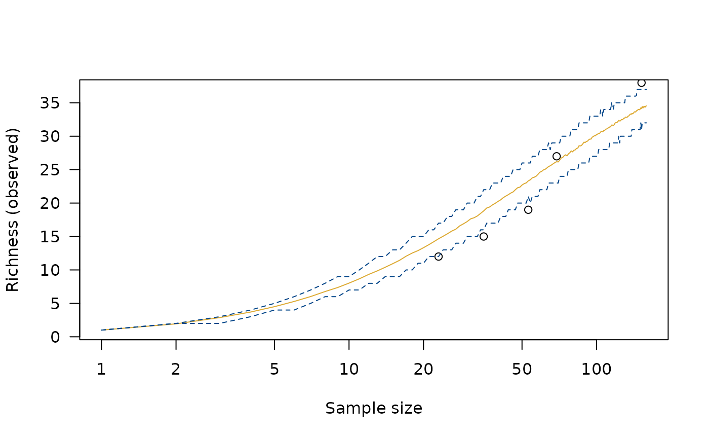
r <- richness(cantabria, method = "observed")
r_sim <- simulate(r)
plot(r_sim)

# }