Similarity

Similarity

Usage

similarity(object, ...)

# S4 method for class 'matrix'
similarity(
  object,
  method = c("brainerd", "bray", "jaccard", "morisita", "sorensen")
)

# S4 method for class 'data.frame'
similarity(
  object,
  method = c("brainerd", "bray", "jaccard", "morisita", "sorensen")
)

Arguments

object

A \(m \times p\) numeric matrix or data.frame of count data (absolute frequencies giving the number of individuals for each category, i.e. a contingency table). A data.frame will be coerced to a numeric matrix via data.matrix().

...

Currently not used.

method

A character string specifying the method to be used (see details). Any unambiguous substring can be given.

Value

A stats::dist object.

Details

\(\beta\)-diversity can be measured by addressing similarity between pairs of samples/cases.

bray, jaccard, morisita and sorensen indices provide a scale of similarity from \(0\)-\(1\) where \(1\) is perfect similarity and \(0\) is no similarity. brainerd is scaled between \(0\) and \(200\).

brainerd

Brainerd-Robinson quantitative index.

bray

Bray-Curtis similarity (a.k.a. Dice-Sorensen quantitative index).

jaccard

Jaccard qualitative index.

morisita

Morisita-Horn quantitative index.

sorensen

Dice-Sorensen qualitative index.

For jaccard and sorensen, data are standardized on a presence/absence scale (\(0\)/\(1\)) beforehand.

References

Magurran, A. E. (1988). Ecological Diversity and its Measurement. Princeton, NJ: Princeton University Press. doi:10.1007/978-94-015-7358-0 .

See also

index_binomial(), index_brainerd(), index_bray(), index_jaccard(), index_morisita(), index_sorensen()

Other diversity measures: diversity(), evenness(), heterogeneity(), occurrence(), plot.DiversityIndex(), plot.RarefactionIndex(), profiles(), rarefaction(), richness(), she(), simulate(), turnover()

Author

N. Frerebeau

Examples

## Data from Huntley 2004, 2008
data("pueblo")

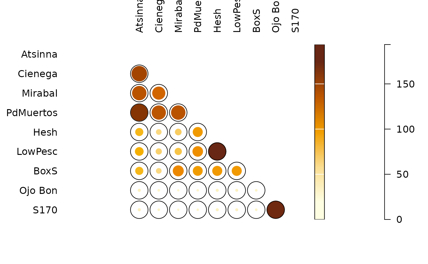
## Brainerd-Robinson measure
(C <- similarity(pueblo, "brainerd"))
#>             Atsinna   Cienega   Mirabal PdMuertos      Hesh   LowPesc      BoxS
#> Cienega   164.36782                                                            
#> Mirabal   152.38095 138.09524                                                  
#> PdMuertos 179.31034 150.57471 152.38095                                        
#> Hesh       82.75862  55.55556  66.66667 103.44828                              
#> LowPesc    89.21023  62.00717  73.11828 109.89989 193.54839                    
#> BoxS       82.75862  55.55556 114.28571 102.17114 103.70370 103.70370          
#> Ojo Bon    27.58621  22.22222  19.04762  20.68966  26.66667  25.80645  22.22222
#> S170       27.58621  22.22222  19.04762  20.68966  26.66667  25.80645  22.22222
#>             Ojo Bon
#> Cienega            
#> Mirabal            
#> PdMuertos          
#> Hesh               
#> LowPesc            
#> BoxS               
#> Ojo Bon            
#> S170      190.53030
plot_spot(C)


## Data from Magurran 1988, p. 166
data("aves")

## Jaccard measure (presence/absence data)
similarity(aves, "jaccard") # 0.46
#>         unmanaged
#> managed 0.4615385

# Bray and Curtis modified version of the Sorensen index (count data)
(sim <- similarity(aves, "bray")) # 0.44
#>         unmanaged
#> managed 0.4442754

# Bray and Curtis dissimilarity
1 - sim
#>         unmanaged
#> managed 0.5557246